Specifications of study area
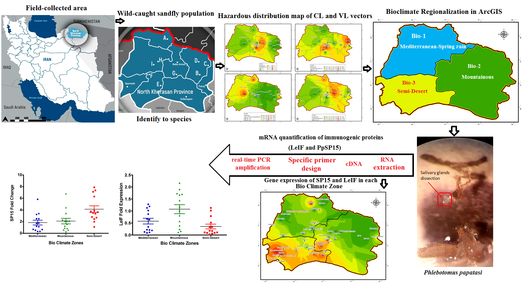
Integrative methods were used to evaluate eco-epidemiological parameters such as bioclimatic change, landscape fragmentation, and ecological niche considering vector domiciliation and their distribution in different locations of Northern Khorasan foci. The Northern Khorasan province is located in northeast of Iran and from the epipaleolithic period onwards was substantially inhabited by nomadic hunter-gathers. Geographic location of studied area (GPS coordinates) is between latitudes of 36˚34 ́-38˚17 ́N and longitudes of 55˚52 ́-58˚20 ́E, and has an area of about 28,434 km2 including eight counties: Bojnord (the capital city of province), Shirvan, Esfarayen, Maneh-o Samalghan, Jajarm, Farouj, Garmeh, Raz-o Jargalan (Fig. 1). This province is bordered Turkmenistan from north, with Khorasan-Razavi province from south and east, with Golestan province from west, and with Semnan province from the southwest (Fig. 1). Northern Khorasan district is generally regionalized into two fractions as: Mountainous areas, and flat regions with low elevation. The Kope-Dagh to the north and Aladagh, extending of the Alborz Mountains to the south, are two main ranges with fertile plains between the mountains, which determine the favorable agricultural conditions and pastoralism. Regarding various weather conditions, this area has a thriving culture and vegetation. Regions of Bojnord, Shirvan, Faruj, and Esfarayen are cold mountainous whereas western districts of Maneh-o Samalghan and Raz-o Jargalan counties are temperate and forested. Parts of lush green forest of Golestan National Park (one of the oldest national parks in the world) are located in Northern Khorasan Province. However, this province has also desert areas such as Jajarm, where there is a wide range of temperature oscillations (cold winters, and relatively hot and dry weather in summer) (Additional file 1: Figure S1a, b, c). Furthermore, significant rainfall amount occurs at different intensities in the province. Due to vast mountainous areas, the Northern Khorasan zone is mainly known to have a cold to temperate mountainous region. The provincial climate is affected by longitude and latitude, and altitude. Also, three basic types of air masses bring variety of weather conditions to the Northern Khorasan area, including (1) Western humid air masses that enters the province in early autumn and lasts until late spring, and the peak of its activity during winter season is the main cause of rainfall in the province (Additional file 1: Figure S1b), (2) Siberian cold air masses, which affects the province from early autumn to early spring causing a significant temperature reduction (Additional file 1: Figure S1c), and (3) a warm dry air mass, which enters to the province from the south during summer, and increased the aridity and temperature (Additional file 1: Figure S1d).
Model variables and climatic regionalization
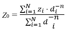
The De Martonne aridity index which is used to determine the regional climate based on annual temperature and rainfall is calculated as follows: I=P/T+10 where (I) stands for De Martonne aridity index, P stands for annual rainfall in millimeters, and T stands for the annual temperature in ˚C (Fig. 1, Additional file 1: Figure S1). Also, climatic regionalization was carried out as earlier described [5] by the use of Principal Component Analysis (PCA) as multivariate statistical method to minimize sources within the variation of the group. Then, Clustering Integration Method (CIM) was applied to precisely improve the classification accuracy. The southern cities have higher temperatures compared to northern regions, due to their different altitudes from sea level, entrance of various air masses, and different longitude and latitudes (Additional file 1: Figure S1). The rainfall levels were also varied in different regions of the province. The maximum and minimum rainfall is observed in spring (March) and summer (June), respectively. Due to highly variability of sand fly species, even in closely distance from its sampled location, we utilized the Inverse Distance Weighting (IDW) deterministic interpolation using ArcGIS 10.3.1 to specify the collected sample points in terms of sand fly dispersion and targeted protein expression rates (SP15 and LeIF) in local scale levels. IDW is a flexible spatial interpolation method, which estimates unknown values along with specifying the search distance, closest points, power setting and, barriers [25]. To obtain the geography map in GIS, ordinary IDW parameters related to the accuracy of the values at each point was calculated with respect to distance: (see Formula 1 in the Supplementary Files)
where Z0 is the estimation value of variable z in point I, zi is the sample value in point I, di is the distance of sample point to estimated point, N is the coefficient that determines weigh based on a distance, n is the total number of predictions for each validation case. The Jaccardʼs similarity coefficient (JSC) is the simplest data, which compares the similarity for two sets of data between different locations of communities. This index always gives a value with a range from the lowest (0%) to the highest similarity (100%) between two populations [26].
Site selection
This cross-sectional study was performed at the peak of sand fly activity from mid-June to the late of September (2017-2018) in the most susceptible biotopes to leishmaniasis where sand flies’ habitats include rural (vegetation, plain and desert fields, and animal shelters), sylvatic-habitats of reservoir hosts (including rodents and dogs) and urban regions (human dwellings). 17 main sites along with surrounding villages were selected from different locations in Northern Khorasan province (Fig. 1, Table 1).
Collecting the Sand flies
Considering geographical locations (altitude, latitude, and longitude) and weather conditions of the counties (Fig. 1, Additional file 1: Figure S1a, b, c, d) as well as during the peak seasons of sand flies activity (according to the incidence of leishmaniasis in each of these regions), trapping was carried out using 120 sticky oil papers, four CDC light traps and, 70 funnel traps. The catching time was from five to 10 days before sunset until sunrise at each location. Dead sandflies were removed from castor oil papers using fine brush and, were put into sterile tubes containing 96% alcohol, and then in order to identify the species, they were kept at -20 ˚C for future morphological and/or molecular experiments. Blood-fed, semi-gravid, and gravid female sand flies were collected alive by the use of aspirator, funnel traps and CDC light traps, and after that were immediately moved into suspended net cages using mouth aspirator. To provide paramount protection of captured sand flies, a piece of 30% sugar-soaked cotton pad was placed on the top panel of holding cages, and were then covered with plastic bags containing a moist sponge to avoid from losing humidity and/or excessive heat. Field-caught sand flies were first euthanized in water, dissected, and were then identified to species based on morphological characteristics of the head and terminal genitalia under compound microscope (400×) using a systematic key [27, 28].
RNA extraction from salivary gland and Leishmania in wild-caught sand flies
Expression pattern of SP15 and LeIF proteins isolated from salivary glands and Leishmania protozoans of P. papatasi were incriminated in different locations of studied areas during the peak of sand fly activity from June to mid-September. Physiological status of sand flies was considered to determine SP15 gene expression level. Therefore, due to fresh-fed sand flies indicated a significant up-regulation of SP15 compared to un-fed ones [29], we selected only blood-fed sand flies to investigate the pattern of expression for SP15 transcript in different eco-epidemiologic conditions of Northern Khorasan province. After accomplishing definitive identification of female P. papatasi, salivary glands in addition to their head accessories were dissected using sterile forceps, and then were immediately re-suspended in 50 μl of RNA-zole® RT solution (MRC, OH, USA), homogenized, and stored at -20°C. To assess the proper expression of SP15, pulled off parts of 10 sand flies were pooled for total RNA isolation (Jena Bioscience, Germany).
To evaluate the expression of LeIF, sand fly-derived metacyclic promastigotes were distinguished by morphology under loop microscope. As parous sand flies (flies that lay eggs) play crucial role in transmitting disease; fresh-fed, gravid, and semi-gravid sand flies were subjected to microscopic examination. Then, the head along with the thoracic midgut forefront which is located in the vicinity of stomodeal valve (SV), and SV area of each infected sand fly were dissected based on the physiological status. Also, parasite isolation from proboscis extending to stomodeal valve of sand fly was not exempt from technical difficulties. Promastigotes obtained from aforementioned area of P. papatasi were counted using Neubauer chamber. The numbers of parasites isolated from each sand fly was approximately 104 promastigotes. RNA Purification was implemented for high yield isolation of total RNA from Leishmania parasites of 10 sand flies with specified status utilizing silica-gel membrane adsorption kit (Jena Bioscience, Germany, http://www.jenabioscience.com) and stored at -80˚C until required. RNA quality and quantity were determined using Nanodrop (BioTek® Synergy™ HTX Multi-Mode, USA).
cDNA synthesis
Complementary DNAs (cDNA) were synthesized as a template for performing quantitative Real-Time PCR (qRT PCR) using the EasyTM cDNA Synthesis Kit (Parstous Biotech, http://www.parstous.com/easy-cdna-synthesis-kit.html, Mashhad, Iran), with respect to the manufacturer’s instructions. Briefly, 8 μl of template RNA from each sample was mixed with kit components in RNase-free tube. After quick vortex, prepared mixture was incubated for 10 minutes (min) at 25˚C, and then was incubated for one hour at 47˚C following stopping the reaction by heating for 5 min at 85˚C, and chilling on the ice for 10 min. To perform PCR or quantitative PCR, the finished RT reaction can be added up to 1/5 of the final PCR volume.
Quantitative Real-time polymerase chain reactions (RT-qPCR)
Real-time PCR reactions were performed to quantify the total amount of SP15 and LeIF transcript expression from salivary gland and Leishmania parasites of P. papatasi sand flies using Maxima SYBRcgreen and Rotor-Gene Q instrument (Qiagen, Germany). The qRT-PCR reactions were set up in duplicates with a total volume of 10 μl , containing 5 μl SYBR green master mix (Fermentas, UK), 0.5 μl each forward and reverse primer (0.8 μM final concentration), 1.5 μl template of cDNA and 2.5 μl Ultra-Pure DNase/RNase-Free water (Invitrogen) in 0.1 ml capillary tubes. Initial reaction was incubated for 10 min at 95 °C, followed by 40 cycles of 95 °C for 15 s (sec), annealing for 30s at 60 °C and extension for 30s at 72 °C. Fluorescent emission was measured at 530 wavelength for SYBR Green dye at the end of the elongation cycle. Expression of SP15 of salivary gland and LeIF of Leishmania gene fragments were assessed in each one of 10 sand fly groups. Each reaction was repeated four times for each gene (in duplicate in two different runs). Quantitative Real-Time PCRs were performed with a 159 bp fragment of the SP15 cDNA using specific primer pairs for SP15 (forward: SP58F, 5′-TGCATTCCCCATTGCAAATATCAG-3′, reverse: SP194R, 5′-AGCACATTCGTGCATAATTTTCC-3′), and LeIF (forward:
LF1014F, 5′-CGTCATCAACTTCGACCTGCC-3′, reverse:
LF1153R, 5′-TCGATCTGCGTGTGGTAGTG-3′) with a 159 bp fragment for the LeIF cDNA. α-tubulin gene was used as a housekeeping load control mRNA to the qPCR reactions primers Tub-P24F and Tub-P24R in P. papatasi sand fly [30]. All PCR experiments were followed by melting curves to check the amplicon specificity.
Different expression ratios for salivary protein and Leishmania genes (SP15 and LeIF) were calculated and displayed as fold changes over a control, using the 2-ΔΔCT method [31]. The fold changes were calculated by the expression 2-ΔΔCT, where ΔΔCT = ΔCT (sample) -ΔCT (calibrator), ΔCT = ΔCT (sample) -ΔCT (alpha tubulin gene), CT = cycle at the statistically significant increase in the emission intensity over the background. The calibrator was represented by the average expression (mean ΔCT) of the newly emergent un-fed nulliparous laboratory-reared female sand flies [30]. Moreover, negative controls were considered without the templates. Fold changes were calculated for each sample in comparison with the calibrator.
Data analysis
Statistical analyses were carried out using the software GraphPad Prism v. 5.01 (GraphPad Software, Inc). Non-parametric KruskalWallis tests were performed to compare the multiple datasets with Mann-Whitney U tests, for accomplishing 2-way pairwise comparisons between data sets when the results for Kruskal-Wallis test were statistically significant, or for comparisons when only two data sets were present. The D'Agostino-Pearson normality test was computed the skewness and then the kurtosis, to quantify how far the distribution is from Gaussian in terms of asymmetry and shape. After that, It calculated how far each of these values differs from the value expected with a Gaussian distribution, and computed a single P value from the sum of these discrepancies. Species biodiversity used in this investigation is affected by two factors as: (1) number of species and (2) their abundance of distribution [26]. Species diversity was calculated based on Shannon-Wiener index, species richness and also evenness index using the Ade4 package of R v.3.5.3 software to estimate the biodiversity of sand fly species in the study areas. Species diversity is a measure of diversity within an ecological community, which encompasses both species richness and evenness of species abundance. Species richness is the number of species in a specific area or environment, whereas, species evenness refers to how close each species are in number in the similar location. Evenness is species abundance distribution and the more even this distribution is the greater the species evenness will be [32]. Computation of these indices is shown in Table 3. Also, estimation by similarity was calculated between different communities using Jaccardʼs similarity coefficient within different localities collection (Table 4).