Observation of seismic signals emitted by wind turbines in the near and far fields
Seismic station TNS is located atop the Kleiner Feldberg (825 m a.s.l.), the second largest peak northwest of Frankfurt am Main, Germany (Fig. 1). Due to its remote location far from highways, industrial areas and railways, the station has a very low noise level of < 10 nm s− 1 and has been providing high-quality data for the permanent monitoring of earthquake activity by the German Regional Seismic Network for more than 3 decades. The Weilrod WF, situated 11 km northwest of station TNS, was erected in 2014 and currently consists of seven Nordex N117 WTs that begin to operate if the wind speed exceeds approximately 3 m s− 1. To measure the frequency and amplitude of the near-field seismic signals emitted by these WTs, an additional temporary seismic station, GSW, was deployed from August 2015 to November 2015 in the centre of the WF. The Taunus mountain range rises to elevations between 200 m and 879 m a.s.l. (the Großer Feldberg being the highest peak). The elevation along a line between GSW at the centre of the WF (source) and TNS (receiver) increases from approximately 450 m to 825 m a.s.l. but fluctuates due to several small valleys.
First, after processing the data (see Methods), we investigate the power spectral density (PSD) to quantify the amplitude of the seismic signals produced by the Weilrod WF at TNS and GSW. The power spectra of the data from both GSW and TNS exhibit peaks at 1.15 Hz and 3.5 Hz, which are correlated with the wind speed (Fig. 2a and 2c). The peak amplitude is increasing with wind speed, which agrees with the report of a recent publication showing that 1.15 Hz and 3.5 Hz spectral noise peaks are typically associated with the operation of Nordex N117 WTs8. However, although the WT-generated signals in the near field (at GSW) are observable between 1 Hz and 10 Hz and even beyond 10 Hz (Fig. 2a), the amplitudes of the three sharp peaks between 2 Hz and 3 Hz at both stations are not increasing with the wind speed, which indicates that their origin is not related to the WTs. Moreover, additional discrete high-frequency (e.g., 6.0 Hz) peaks are observed at the near-field station (GSW), whose data are dominated by the WT-emitted signals (GSW is only 150 m from the closest WT), whereas this peak is not identified at TNS. These observations support the assumption that the two spectral peaks at 1.15 Hz and 3.5 Hz observed at TNS are associated with the operation of the Weilrod WF but are reduced in amplitude relative to those at GSW due to the decay of wave energy with increasing distance from the WF. Signals beyond 3.5 Hz that are detectable at GSW are not observable at TNS, due to attenuation and geometrical spreading effects and therefore are not considered further in the modelling.
Next, to better quantify the spectral noise amplitudes of the WF signals with 1.15 Hz in terms of maximum ground velocities at GSW and TNS (Fig. 2b and 2d), we determine the I9518 values (95.45% of the amplitudes are within two times the standard deviation) of the bandpass-filtered signals with cutoff frequencies of 1 Hz and 1.4 Hz. For each station, we select a one-hour time segment with a wind speed < 0.5 m s− 1 and another one-hour time segment with a wind speed > 9 m s− 1. The I95 noise amplitudes at GSW (TNS) in the near (far) field are approximately 240 nm s− 1 (15 nm s− 1) at a high wind speed and 52 nm s− 1 (7 nm s− 1) at a low wind speed. We conclude that at high wind speeds and within the frequency range of 1 Hz − 1.4 Hz, the Weilrod WF, on average, causes a 2.1-fold increase (from 7 nm s− 1 to 15 nm s− 1) in the noise level at TNS and that the seismic signals produced by the Weilrod WF are detectable in 11 km at TNS, because of the overall low noise level at TNS.
Model setup for simulating the seismic signals from WTs
The numerical simulations are based on a 3D model (17 km x 19 km) of the uppermost crust (depth of 3.2 km) and surface topography in the region around the Weilrod WF and station TNS (Fig. 1). The model is a homogeneous half-space characterized by isotropic physical properties (no geological layering). We assign a uniform shear-wave velocity of vS=1800 m s− 1 and compressional-wave velocity of vP=1.7 vs, and the density is set to 2600 kg m− 3. In a first step, anelastic absorption (attenuation) of waves is not included in the model to focus on topographic effects. However, further below we will include attenuation effects by specification of the seismic quality factors QS (for S-wave propagation) and QP (for P-Wave propagation). The location of the source is set on the surface at the coordinate of one of the seven WTs in Weilrod (WT4 in Table 1). The source features a vertical component (Z) only to simulate an up- and downward motion at the foundation of the WT. A receiver is located at the location of TNS to extract synthetic waveforms during the numerical forward modelling. For the source time function, we sum three sinusoidal functions with frequencies of 1.15 Hz, 3.50 Hz and 6 Hz (each with a duration of 5 s), which correspond to the characteristic frequencies of the three peaks measured at GSW and TNS (Fig. 2a and 2c). The topography in the model is defined based on a digital elevation model (DEM) using data with a resolution of 30 m from the Global Multi-Resolution Topography (GMRT) synthesis project19.
Simulating synthetic waveforms at TNS
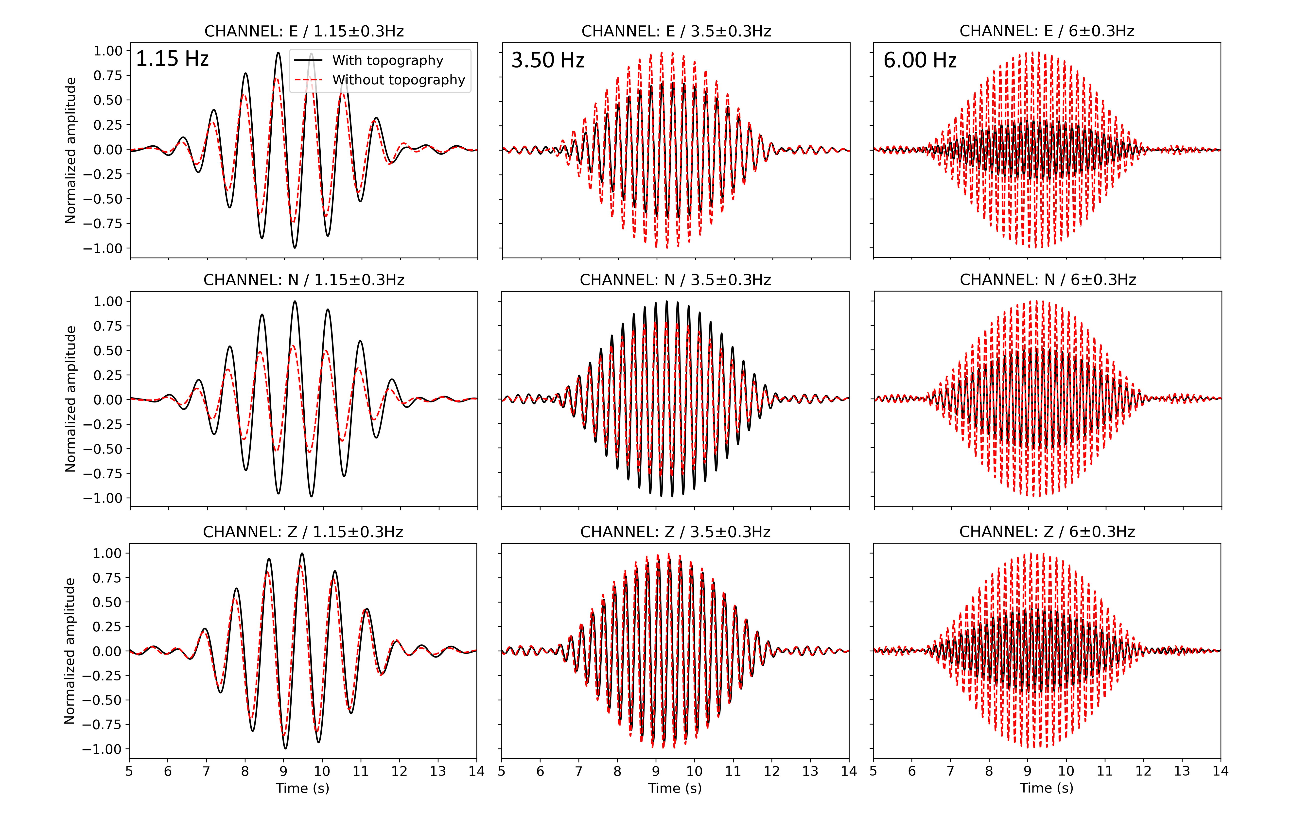
To study the effects of topography on the signal amplitude at TNS, we perform simulations in an isotropic half-space model (see Methods) both including and excluding topography. To simulate wave propagation, we use the software package Salvus20 provided by Mondaic AG/Ltd in Zurich, Switzerland. The Z, N (Y) and E (X) components of each synthetic seismogram at TNS are bandpass filtered in three frequency bands: 1.15 ± 0.3 Hz, 3.5 ± 0.3 Hz and 6.0 ± 0.3 Hz. By comparing the two model simulations with and without topography, we find that including topography reduces the signal amplitudes on all components of the 6.0 Hz signal and the Z and E components of the 3.5 Hz signal (see supplements Fig. S1), which can be explained by the scattering and reflection of waves along their paths. In contrast, the amplitudes on the N component of the 3.5 Hz signal and on all three components of the 1.15 Hz signal are greater with topography than they are without topography (see supplements Fig. S1), indicating that topography has an amplifying effect on WT-emitted signals at comparatively low frequencies. While high-frequency waves particularly suffer from scattering due to topography, low-frequency waves seem to be focused and modulated in a constructive manner along their travel path; this amplifying effect is observed in a similar way concerning earthquake waves16,17.
Radiation from a single wind turbine
Here, to further investigate the spatially varying effects of topography on low-frequency signals, we simulate and analyse the propagation of surface waves at 1.15 Hz (the dominant frequency of the signals emitted by the WTs) using a 1.15 Hz sinusoidal source time function and generate maps of the vertical peak ground velocity (PGV) both with and without topography (Fig. 3a and 3b). In both cases, we use a single WT at the centre of the Weilrod WF as the source. For both model setups, we plot the spatial distribution of the topographic amplification factor A (Fig. 3c) by calculating the signal amplification or reduction in percent (%) based on Eq. 116:
$$A=\left(\frac{{PGV}_{w}}{{PGV}_{wo}}-1\right)\times 100$$
1
where PGVw denotes the PGV obtained with topography and PGVwo denotes the PGV obtained without topography. The map of the resulting amplification factor A (Fig. 3c) indicates that the amplitudes of 1.15 Hz signals are significantly modulated by topography. This effect is especially pronounced on the mountainside to the south–southeast of TNS and Großer Feldberg, reflecting the apparent correlation between the reduction and amplification of the PGV with the DEM. In contrast, the mountain ridge between the WT source and TNS appears to act as a wave guide and preserves the signal amplitude along its path, thus opposing the expected reduction with geometrical spreading. Generally, however, the PGVs decrease with increasing distance from the WF. Even for a single WT in Weilrod, however, we can demonstrate the amplifying effect of the topography on the signal amplitude near TNS.
Radiation from multiple wind turbines considering the effects of wavefield interference
The wavefield of a single WT can differ significantly from the complete wavefield of an entire WF due to constructive and destructive interference8. To consider these effects in detail, we expand our study and place a source at each of the 7 WTs in the Weilrod WF and numerically simulate 100 PGV maps without topography using a randomly chosen signal phase of the sinusoidal time function for each of the seven sources. The modelling results show both destructive interferences, resulting in a low PGV at TNS (Fig. 4a), and constructive interference, yielding relatively high PGVs (Fig. 4b). Since the WTs are not all expected to vibrate in phase, a single interference pattern can represent only a snapshot of the ground motion before the radiation generates another pattern. Therefore, to derive a representative radiation pattern, we averaged 100 different PGV maps (Fig. 4c), thereby avoiding the domination of any single interference pattern. The resulting average PGV map (Fig. 4c) shows the decrease in amplitude with increasing distance from the WF, but the obtained pattern differs clearly from the two patterns with either only destructive interference or only constructive interference.
Radiation from multiple wind turbines considering the effects of wavefield interference, topography, and attenuation
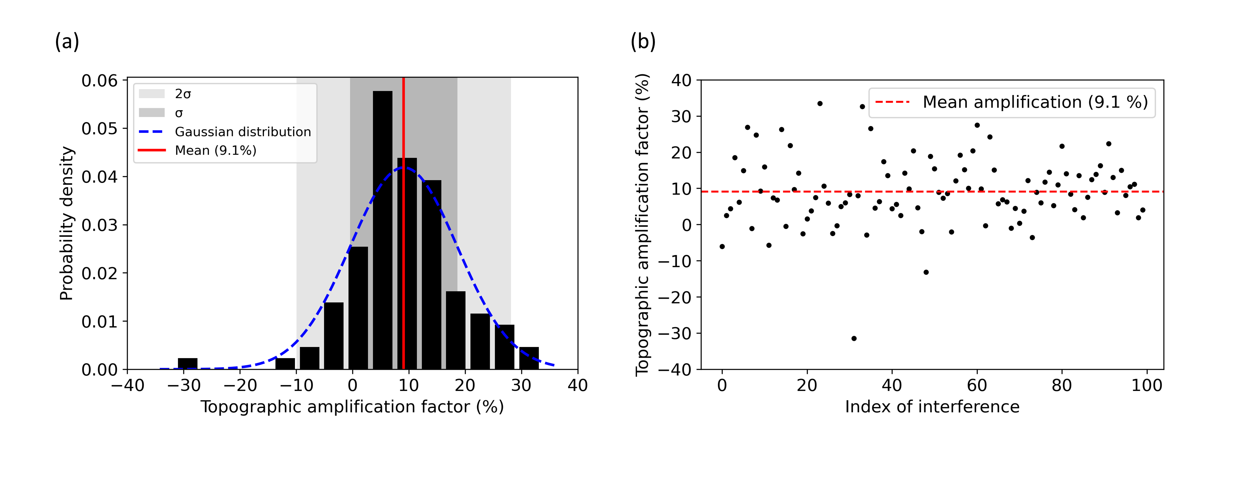
Finally, we calculate the average PGV distribution produced by the whole Weilrod WF considering both the effects of topography and the interference caused by the emissions of multiple WTs (Fig. 5a). The same set of randomly chosen phases of the source time functions used for the case without topography (Fig. 4c) is used again in this case, and 100 individual PGV maps are averaged, allowing us to compare the average PGV distributions obtained without (Fig. 4c) and with (Fig. 5b) topography. In the same manner as Fig. 3c, a map of the PGV amplification factor is obtained (Fig. 5b), the distribution of which reveals that amplitudes are preserved along the mountain ridge between the WF and TNS if topography is included in the model. The minimum amplification factor in the study area is -20% (an amplitude reduction of 20%), while the maximum value is 30% (inset in Fig. 5b); however, such high amplification factors (values > 20%) are limited to a small proportion (< 1%) of the total area. Generally, the map of the amplification factor is comparable to that in the scenario with only a single WT (Fig. 4c), although considering all seven WTs causes some amplification areas to be enlarged, generally along the mountainsides facing away from the source (e.g., to the south of TNS and Großer Feldberg, similar to Fig. 4c). In contrast, amplitude reductions are associated mostly with valleys16. By comparing the synthetic waveforms at TNS for each of the 100 interference scenarios with and without topography, we infer that the amplitude at TNS increases by approximately 9% on average if topography is considered (see supplements Fig. S2). Generally, with respect to the 100 specific interferences, an amplification due to the topography near TNS is much more likely than a reduction (see supplements Fig. S2).
To further investigate the decay of the PGV, we extract the PGVs along a straight line connecting the location of GSW to TNS and plot the simulation results both including and excluding topography (Fig. 5c). The amplitude steadily decreases logarithmically with increasing distance from the WF if topography is not included, as expected, whereas the amplitude decreases globally with topography but increases locally (e.g., at distances of 4–5 km, 6–8 km and 11–15 km). The sudden increase of amplitudes at a distance of 500 m is observable for the case with and without topography and is likely a consequence of wavefield interferences. In case of attenuation using QS=25 and QP=40, the amplitude decay with distance is higher; however, the local topographic effects remain. As mentioned before, the amplitudes significantly increase on the mountainside behind TNS opposite the WF. The PGVs along the line are calibrated to the noise amplitude (I95) of approximately 240 nm s− 1 measured at GSW for wind speeds > 9 m s− 1 (Fig. 2b). This means that the simulated amplitude at the location of GSW is matched up with the I95 value measured at GSW. Furthermore, we measure an amplitude (I95) of approximately 15 nm s− 1 at TNS at wind speeds > 9 m s− 1 (Fig. 2d). The resulting simulated amplitude including the effects of interferences, topography, and attenuation fits well with the observed amplitude of 15 nm s− 1 at TNS, which means that the measured amplitude at TNS is predictable if these effects are included. Overall, this analysis demonstrates that the amplitude of noise at TNS (and other areas in the Taunus region) caused by low-frequency WT signals is underestimated if topography is neglected in the model.