Study area and working units: this study is conducted at the scale of the European continent (supplementary Fig. 11). We classified all pixels within Europe using the GLDAS Vegetation Class/ Mask40 (GVC, see supplementary Fig. 11). The GVC map is available at https://ldas.gsfc.nasa.gov/gldas/vegetation-class-mask. To classify the pixels, dominant GVC land cover types were selected for further analysis. Selected land cover types include croplands, evergreen needleleaf forests, mixed forest, open shrublands, wooden tundra, grasslands, and mixed tundra. Once the work units were identified, all calculations were performed on a pixel-by-pixel basis and then the results within each work unit were averaged (wherever necessary) to obtain class-specific results.
Datasets: Data from different sources are used for this analysis. We used NDVI (Normalized Difference Vegetation Index) data from the Global Inventory Monitoring and Modelling System (GIMMS) 26,27(covering the period 1981-2015), the Advanced Very High-Resolution Radiometer (AVHRR)28 (covering the period 1981-2020), and the Moderate Resolution Imaging Spectroradiometer (MODIS) 29 (covering the period 2001-2020) to determine the OG and OD and consequently the LGS. In addition, the NASA Global Land Data Assimilation System (GLDAS) along with the NOAH Land Surface Model39-41 (v2.0, for 1982-2014, and v2.1, for 2000-2020), the European Centre for Medium-Range Weather Forecasts (ECMWF) ERA5- land42 (for 1982-2020), and the Global Land Evaporation Amsterdam Model43,44 (GLEAM v3.6a, for 1982-2020) were the three other datasets used in this analysis. We also used in situ measurement data from FLUXNET45 (with a duration of 1995-2020) as a benchmark for the reanalysis data.
Data preprocessing: The data used in this analysis from different sources are provided at different spatial resolutions, with the coarser resolution being 0.25 degrees for GLDAS and GLEAM databases. Therefore, for consistency, we used the RegularGridInterpolator function of the interpolate sub-package of the Python package of scipy to interpolate them (wherever necessary) with a resolution of 0.25 degrees, using the same latitude and longitude vectors of the GLDAS and GLEAM databases. In the case of the NDVI data, we used the GIMMS NDVI data as a benchmark for our analysis because it is commonly used in other studies. However, it should be noted that the GIMMS NDVI data are available at biweekly temporal resolution (i.e., two data per month), the MODIS NDVI data are available at monthly resolution, and the AVHRR NDVI data are available at daily resolution. Therefore, we brought them all to monthly resolution by averaging the data that fall within each month, i.e., in the case of the GIMMS data, the two data within each month, and in the case of the AVHRR data, all daily data of each month. This was necessary because the temporal resolution of the NDVI data affects the derived OG and OD values. Additionally, we excluded the last three years of AVHRR data (2018-2020) from the analysis due to unknown quality of the data for these years.
The Princeton meteorological forcing data used for GLDAS 2.0 ends in 2014, so GLDAS 2.1 (covering 2001-present) uses other forcing data including observation-based P and solar radiation, resulting in significantly higher values nearly for all variables, as the climatology of the forcing variables differs from that of the Princeton forcing dataset. Therefore, we used the overlapping period 2001-2014 to construct location- and day of year-specific linear regressions between paired variables from v2.0 and v2.1, and then applied the developed regression to match the GLDAS 2.1 data to the climatology of GLDAS 2.0. In the case of P, day of year-specific linear regressions were not possible due to high variability and frequency of zero values, therefore we only applied site-specific linear regressions.
While the temporal resolution of the GLEAM dataset is daily, the GLDAS data are provided with a temporal resolution of 3 hours. Therefore, we averaged the 3-hourly data from GLDAS to account for the daily data. Although the ERA5-land dataset is originally provided with a spatial resolution of 0.05 degrees and a temporal resolution of 1 hour, for consistency, we downloaded the daily and 0.25-degree resolution data using the ERA5-land Daily Statistics CDS API[1].
In cases where a variable was available from two or more of the above reanalysis products, a PCA was performed, and the first component was then used for further analyses when the target variable was in demand. This was the case for ET and SSM. In the case of ET, the first component accounted for 95 or more percent of the variation in all products, while in the case of SSM, 85 or more percent of the variation in the products used was explained by the first component.
Data validation: Before any further analysis, we validated the ET and SSM data from the datasets used (GLDAS, GLEAM and ERA5-Land) by comparing them with in situ measurement data from FLUXNET45. For this purpose, we extracted reanalysis data on ET and SSM for the pixels containing FLUXNET stations for the overlapping periods 2000-2020, and then performed a station-by-station comparison of the reanalysis data with the FLUXNET data. In total, 8 and 23 FLUXNET stations contain the complete data for ET from all datasets for the 2000-2009 and 2010-2020 periods, respectively, while only 4 and 18 stations have the complete data for SSM from all datasets for the 2000-2009 and 2010-2020 periods, respectively. Supplementary Fig. 12 shows the Pearson correlations between ET and SSM from FLUXNET and ET and SM from other datasets. There are strong correlations between ET from FLUXNET and ET from GLDAS, GLEAM and ERA5-land with correlation coefficients ranging from 0.59 to 0.87 for the period 2000-2009 and 0.64 to 0.91 for the period 2010-2020. In contrast to ET, the correlations between SSM from FLUXNET and SSM from GLDAS, GLEAM and ERA5-land appear to be weak (with correlation coefficients ranging from 0.24 to 0.60 for the period 2000-2009 and 0.07 to 0.83 for the period 2010-2020), partly due to the uncertainty of SSM measurements at FLUXNET stations, as seen in the large changes in SSM values or repeated constant values for some months. Overall, it seems that the reanalysis data used in this investigation can reasonably show the ongoing trend in the real world, and we can be confident that the conclusions we have drawn in this paper are valid.
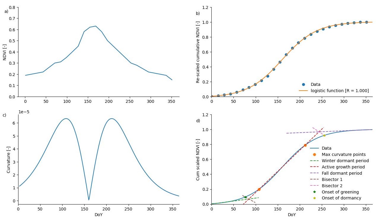
LFD NDVI Method: To determine the OG and OD for individual pixels in Europe and for individual years of the entire study period (1982-2020), we needed an innovative algorithm that could operate independently for each year and pixel. This was important because classical methods, e.g., Piao et al. 53, typically calculate a critical long-term NDVI value for the entire period and then determine the timing for approaching such a critical value in all individual years. However, this was prone to bias because the NDVI data used came from three different products of GIMMS [1982-2015], AVHRR [1982-2017], and MODIS [2001-2020], especially with different temporal resolutions (biweekly, daily, and monthly), which can affect the long-term critical value and consequently the timing for OG and OD. Therefore, we developed the logistic function derivative of NDVI curve (LFD NDVI method) which can be used for each year individually. It uses the first and second derivatives of the fitted logistic function of the cumulative NDVI curve of a given year to determine the OG and OD (Extended Data Fig. 1a). As a first step, we converted all data to a monthly time scale, as mentioned earlier. Then we calculated the cumulative NDVI data over time and finally fed them into the LFD NDVI method to determine OG and OD. However, before feeding the data into the LFD NDVI method, we normalized both the NDVI and time data between 0 (min) and 1 (max) as this was required for further calculation. Normalization of the NDVI data was done twice, once before accumulation to eliminate possible negative NDVI values, and another time after accumulation to bring them within the range of 0 to 1. In the following, the calculation with the LFD NDVI method is described in detail. When t and NDVI are referred to in the following, the rescaled forms are meant for the sake of simplicity.
In a first step, a logistic function was fitted to the data (Extended Data Fig. 1b):
$$y\left(t\right)=a+ \frac{b}{1+\text{e}\text{x}\text{p}(-\frac{t-c}{d})}$$
1
where y(t) is the cumulative NDVI on day t of the year and the model coefficients are a, b, c, and d. Using this fitted function, we obtained the smoothed curve of the cumulative NDVI data for all days of the year (t = 1:365 or 366, being scaled to 0 and 1). Third, we determined the curvature of the data, k(t), for each t using the first y'(t) and second y''(t) derivatives of the fitted logistic function:
$$k\left(t\right)=\frac{\left|y{\prime }{\prime }\left(t\right)\right|}{{\left(1+y{\prime }\left(t\right)\right)}^{1.5}}$$
2
Plotting k(t) versus t typically showed two maxima separated by a minimum. The times at which the maxima occur allow the logistic curve to be divided into three parts with nearly linear behavior (Extended Data Fig. 1c). The first part occurs during the winter and early spring before the first curvature maximum in the data; we refer to this part as the winter dormant period. The second part occurs between the first and second curvature maxima in the data; we refer to this part as the active growth period. Finally, the third part occurs during the late summer and fall after the second curvature maximum in the data; we refer to this part as the fall dormant period.
For the second part, a first-order polynomial function was fitted by simply using the two points of maximum curvature and their respective cumulative NDVI values, plus an additional point in between. For the first and third parts, we used the sequential linear approximation method described by Dathe et al. 54 to identify the linear part of the rescaled cumulative NDVI curve before the first and after the second curvature maximum. The method consists in calculating linear regressions over a consecutive number of points before the first and after the second curvature maximum. The dependence of R2 on the number of data points was used to determine the number of points to be included in the regression. In this analysis, an R2 value of 0.95 was used as the critical value to determine the linear parts of winter- and fall-dormant. Next, we determined the equation of the bisector of the obtuse angle between the regression equations of the winter-dormant and active growth parts (Eq. 3) and the fall-dormant and active growth parts (Eq. 4) by computing the angle between two lines.
$$\text{y}\left(\text{t}\right)={a}_{\text{w}\text{a}}t+{c}_{\text{w}\text{a}}$$
3
$$\text{y}\left(\text{t}\right)={a}_{\text{f}\text{a}}t+{c}_{\text{f}\text{a}}$$
4
where awa and cwa correspond to the slope and intercept of the line bisecting the lines of winter dormancy and active growth parts, and afa and cfa correspond to the slope and intercept of the line bisecting the lines of fall dormancy and active growth parts. After determining the equations for the bisecting lines, the intersection between them and the fitted logistic function determines the OG and/or OD (Extended Data Fig. 1d). Mathematically, OG and OD are calculated by solving the following equations for t:
$${a}_{\text{w}\text{a}}t+{c}_{\text{w}\text{a}}=a+ \frac{b}{1+\text{e}\text{x}\text{p}(-\frac{t-c}{d})}$$
5
$${a}_{\text{f}\text{a}}t+{c}_{\text{f}\text{a}}=a+ \frac{b}{1+\text{e}\text{x}\text{p}(-\frac{t-c}{d})}$$
6
In this analysis, the root_scalar function of the Optimize sub-package of the Python package scipy (as an alternative to the "fzero" function in MATLAB) was used to find a null of the above expression by changing the t values.
Using the above-mentioned method, we determined the OG and OD from three different NDVI products of the GIMMS (for the period 1982–2015), the AVHRR (for the period 1982–2017), and the MODIS (for the period 2001–2020). Since the higher quality of GIMMS data is already well documented, we used the results obtained with GIMMS as a benchmark and compared the results from two other products to it. A scaling factor at different land use levels was used to adjust the results of the AVHRR and MODIS to GIMMS. Finally, the average values for the OG and OD from these products were used for further analysis.
Trend analysis of Mann-Kendall test: In this analysis, we examined the overall trend of OG and OD as well as LGS using the Mann-Kendall test30,31. To do this, we applied the Python implementation of the nonparametric Mann-Kendall trend analysis called pyMannkendal55 employing the original and Theil-Sen methods with a significance level of 0.05. Both original and Theil-Sen methods show how the OG, OD, and/or LGS change with time, but Theil-Sen is more robust against individual outliers56. As suggested by Cortés et al. 56, prior to trend analysis, we dealt with temporal autocorrelation of data with AR(1)correction to prevent the occurrence of false positive rates57. As suggested by von Storch 57 and outlined by Cortés et al. 56, the following equation is used to calculate the temporal autocorrelations at lag -1:
$$\widehat{r}=\frac{n{\sum }_{1}^{n-1}\left({x}_{t}-\stackrel{-}{x}\right)\left({x}_{t+1}-\stackrel{-}{x}\right)}{\left(n-1\right){\sum }_{1}^{n}{\left({x}_{t}-\stackrel{-}{x}\right)}^{2}}$$
7
where \(\widehat{r}\) is autocorrelation, xt is data at time t, \(\stackrel{-}{x}\) is the mean value of all data, and n is number of the data. Then, when autocorrelation is computed, the original time series (xt) were replaced with adjusted one (yt) using following equation:
$${y}_{t}={x}_{t}-\widehat{r}{x}_{t-1}$$
8
Group Method of Data Handling: we applied the group method of data handling (GMDH) 38 to develop a gray box network predicting the OG and OD, and the LGS, using several meteorological variables along with soil moisture as inputs. For this purpose, we used the main meteorological variables (T, P, and VPD) plus SSM and RSM. We excluded ET and transpiration from this analysis because they are logically strongly correlated with the phenological states of vegetation and mask the importance of other variables. We also excluded climate indices (NAO: North Atlantic Oscillation, El Nino, etc.) from this analysis because the pretest showed that in this context, they play a lesser role than the other included variables. All included variables were averaged for several time periods, namely winter [January 1 to 30 days before the OG], early spring [30 days before the OG to the OG], spring [OG to the PG], summer [PG to the two weeks before the OD], and late summer [two weeks before OD to the OD]. Then, their long-term anomalies were calculated for each period and then subjected to modeling.
The following quadratic regression is used to obtain the preliminary estimates (zij) for the first layer of the GMDH network58:
$${z}_{ij}={c}_{0}+{c}_{1}{x}_{i}+{c}_{2}{x}_{j}+{c}_{3}{x}_{i}^{2}+{c}_{4}{x}_{j}^{2}+{c}_{5}{x}_{i}{x}_{j}$$
9
where xi and xj represent the pairwise selection of input variables and c0 to c5 represent the polynomial predictors. The following equation determines the total number (n) of possible polynomials58:
$$n=\frac{N\times (N-1)}{2}$$
10
where N is the number of input variables. To develop the GMDH network, we first developed all possible polynomials with pairwise selected variables (xi and xj). Then we had to filter out the least effective new variables using a statistical selection criterion38. We used the following criteria to select the best new variables to build the next layer of the network59:
$$e=p\times RMS{E}_{\text{l}\text{o}\text{w}\text{e}\text{s}\text{t}}+(1-p)\times RMS{E}_{\text{h}\text{i}\text{g}\text{h}\text{e}\text{s}\text{t}}$$
11
where p is the selection pressure and means a number between 0 and 1 (with p = 0.75 in our analysis), with higher numbers indicating higher pressure in selecting new variables. The preliminary estimates with root mean square error (RMSE) smaller than e were selected for the next layer. The polynomials were then further improved by repeating steps 1 and 2 and using new selected variables (zij) from the previous step. This continues until the smallest value of the selection criterion from the current iteration shows no improvement over the smallest value from the previous iteration58.
To develop GMDH models for predicting anomalies in LGS (the same applies for the OG and OD), we forced the models to have only one layer with two most important variables going into the model. The concept underlying this strategy is to select only two variables for each pixel for predicting the OG and OD or the LGS. To train and evaluate the developed networks, the data were randomly split into two subsets, with 70 percent of the data used to train the networks and the rest used to test as independent data.
The GMDH method provides a built-in algorithm58,59 that retains only the essential input variables. Therefore, here we repeated 100 times the random division of the data into training and test subsets, developed the models, and calculated the Pearson correlation (R) between the target and output variables for each replication. Then, the replications with R value less than 0.7 in the evaluation subset were filtered out and the selected sets of variables for predicting the onset of the OG and OD and LGS in the remaining replications were determined. The used GMDH algorithm is coded in Python.
To visualize the results obtained from GMDH analysis, the first and second important control factors of anomalies of LGS (as well as OG and OD) are plotted against each other, and the colors show their frequency among the pixels in Europe (see supplementary Figs. 6 and 7). In this way, we were able to check which variable was the most important factor and with which other variable it usually paired to explain the anomalies in LGS (and/or OG and OD).
Principal component analysis and biplotting: To investigate the direction of the effects of the control factors on LGS as well as OG and OD, we performed PCA on the data and illustrated the result as biplots. Biplots show both the observations and the original variables in principal component space60. In a biplot, positively correlated variables are closely aligned, while negatively correlated variables are aligned in the opposite direction. In both cases, the stronger the correlation between variables, the larger the size of the arrows. Variables aligned at 90 degrees to each other have no correlations 61.
[1] - https://cds.climate.copernicus.eu/cdsapp#!/software/app-c3s-daily-era5-statistics?tab=overview
References
53 Piao, S., Fang, J., Zhou, L., Ciais, P. & Zhu, B. Variations in satellite-derived phenology in China's temperate vegetation. Global change biology 12, 672–685 (2006).
54 Dathe, A., Eins, S., Niemeyer, J. & Gerold, G. The surface fractal dimension of the soil–pore interface as measured by image analysis. Geoderma 103, 203–229 (2001). https://doi.org/10.1016/S0016-7061(01)00077-5.
55 Hussain, M. & Mahmud, I. pyMannKendall: a python package for non parametric Mann Kendall family of trend tests. Journal of Open Source Software 4, 1556 (2019).
56 Cortés, J. et al. Where are global vegetation greening and browning trends significant? Geophysical Research Letters 48, e2020GL091496 (2021).
57 von Storch, H. in Analysis of Climate Variability. (eds Hans von Storch & Antonio Navarra) 11–26 (Springer Berlin Heidelberg).
58 Pachepsky, Y. A. & Rawls, W. Accuracy and reliability of pedotransfer functions as affected by grouping soils. Soil Science Society of America Journal 63, 1748–1757 (1999).
59 Rahmati, M. Reliable and accurate point-based prediction of cumulative infiltration using soil readily available characteristics: a comparison between GMDH, ANN, and MLR. Journal of Hydrology 551, 81–91 (2017).
60 Gabriel, K. R. The biplot graphic display of matrices with application to principal component analysis. Biometrika 58, 453–467 (1971).
61 Rahmati, M. et al. Development and analysis of the Soil Water Infiltration Global database. Earth System Science Data 10, 1237–1263 (2018).https://doi.org:10.5194/essd-10-1237-2018.