In this paper, the risk of hypertension is modeled using the PRS and CNN methods. These models use SNP and age without any clinical factors.
Polygenic risk score
Because a person's genomic does not have significant changes from birth, genomic information can act as an early predictor of risk. Hypertension is affected by several genetic variants with small effect sizes. It is necessary to examine the mass effect of multiple SNP by calculating a single metric that represents an individual's overall genetic risk score to predict significant risk. A simple genetic risk score (GRS) is a simple sum of the number of risk alleles (usually several SNPs from GWAS, sometimes based on weight-effect measures) present in each individual (22). Recently, a wide range of SNPs, from thousands to millions of SNPs, have been used to create an improved GRS such as PRS (23).
The size of the risk presented by PRS is a possible range, and this differs from risk information from genetic markers of single-gene disorders.
Plink and gcta64 software are used to calculate PRS. The execution code is as shown in Fig. 1. It should be noted that the execution of code on files in the ped format that stores genomic data, is executed on the Linux platform.
In addition, to validate the model, the data is divided into test and train, and the PRS calculated separately and finally used in the disease prediction model.
Convolutional neural network
A convolutional neural network is suitable for processing data with two properties: (1) spatially related properties, such as an image with pixels arranged in an array or a video with images in a row. (2) Features are homogeneous across the page. The main structure of CNN consists of input layers in an image page.
Other layers include the convolution layer, the pooled layer, the fully connected layer, and the output layer (24). The convolution layer extracts local features based on the weight of the neurons by entangling all parts of the image. The pooled layer performs independent operations on each feature map, such as average or maximum integration, which can effectively reduce the resolution of the feature and reduce the number of network parameters required for optimization. CNN puts these basic structures together and puts the first layer as the input of the second layer, which can learn deeply. CNN implementation steps are shown in Fig. 2.
The first step is converting the genome data stored in a ped file to an image file. To do this, in every 4 pixels in a row, only one cell is blacked out based on the genome type, and the rest of the cells remain white. For best input, the length and width of the image are considered equal to the square of the number of genomes, which is equivalent to 600K SNPs. This method reduces the volume of genomic data with a compression factor of 13%. In the next step, a deep network based on the convolution layer with 24 filters is formed. The filters are 4 * 4, in which only one column in each row has a value of one and the rest is zero, and after applying the filter, the results are pooled. The number of CNN layers depends on the complexity. In this study, six layers are appropriate. After each convolution layer, the max-pool layer is 2 * 2, which reduces the image's dimension in length and height. Due to the different inputs, the data is normalized after six layers. Finally, the image is converted into an array and input to the FCN. The sample image is shown in Fig. 3 after six layers.
Research data
The research data consists of genomic data, age, and longitudinal data of blood pressure phenotype for 7268 participants in six phases. These data were selected from the Cardiac-Metabolic Genetics Study of Tehran (TCGS) (25). TCGS is a genetic cohort study to determine the risk factors for major non-communicable disorders in the Tehran Lipid and Glucose Study (TLGS) (26).
This research with the code IR.SBMU.ENDOCRINE.REC.1400.008 was approved by the National Ethics Committee in Biomedical Research in May 2021. All participants provided a sufficient baseline blood sample for plasma and DNA analysis and gave written consent for blood-based analysis and long-term follow-up. All methods of this study were performed according to appropriate and relevant instructions. All participants were included except those with isolated diastolic blood pressure (DBP greater than 90 and SBP less than 140 mmHg) (27). To measure blood pressure, participants first sit in a chair for 15 minutes, after which their specialist measures their blood pressure twice using a standard mercury sphygmomanometer. There is at least a 30-second interval between these two separate measurements, and the average of the two measurements is recorded as the participant's blood pressure (28).
Individuals who have an SBP above 140, a DBP above 90, or a participant taking hypertension medication at any phase are labeled hypertensive and otherwise considered normal (19, 29).
In phase two or three, genome samples from white blood cells were genotyped by standard proteinase K method extracted with HumanOmniExpress-24-v1-0 chip by deCODE according to Illumina device (30). Genomic data for each individual has 600K SNPs stored in the ped file.
Based on (31) to improve results and quality control, classification based on age (over 18 years and under 18 years) and SNP classification has been done in rarity and prevalence. Accordingly, SNPs with missing values less than 5% and mean allelic frequency (MAF) greater than 5% are considered.
Validation and evaluation of results
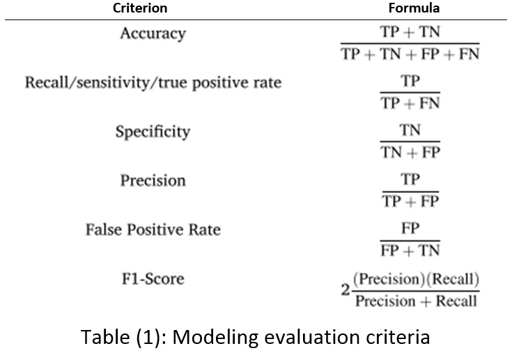
Various criteria are expressed in the subject literature to validate and evaluate modeling results, shown in Table 1. TP, TF, FP, and FN stand true positive, true negative, false positive, and false negative. These criteria express the efficiency of the constructed model in the research data.
In addition to these criteria, one of the most widely used criteria to compare models is the area under receiver curve (AUC). A complete classification will have an AUC of 1, and a weak classification will have 0.5. A good classifier will have an AUC greater than 0.5 and is considered excellent when it reaches 1 (32).
The 10-fold method is used for modeling validation, which divides the data into ten equal parts without repetition and creates different models, calculating the final result based on the average of the obtained results. It should be noted that because there is similar data in phases for each participant, all rows for one participant are in only one fold.
PHP language is used to prepare the data, and Orange is used for modeling and visualizing. The code and sample data are placed on Github.