Study design and data resource
We conducted an ecological study using secondary open data published as government statistics for 2010, 2013, and 2016 by prefecture. The data used for analysis were LE, three measures of HLE, population by age, number of deaths, and the number of unhealthy people. Values of HLEs and LE were obtained from the “Healthy Life Report from Japan.”3 All other variables were derived from the government statistics website, “e-Stat.”15 The population by age was derived from the population census for 2010, and population estimates for 2013 and 2016. The number of deaths was derived from official vital statistics. There are three measures of unhealthy people for each HLE (Additional file 1). The people who answered “Yes” to the question “Do health problems currently affect your daily life in some way? (Yes/No)” for DFLE-AL, and the people who answered “Not very good” or “Not good” to the question “What is your current state of health?” on a 5-point scale rating (not good–very good) for LE-SH, were regarded as unhealthy. The data for these two questions were derived from a comprehensive survey of living conditions.16 In DFLE-CN, people requiring long-term care (level 2 or higher) were determined to be unhealthy in a survey of long-term care benefit expenses.17 In the analysis, these variables were converted to the following rates or ratios: aging rate, mortality, and proportion of unhealthy people.
Main outcome
LE and three measures of HLE were used as outcome variables.
Main predictors
The proportion of unhealthy people was used as the main predictor. In this paper, we defined the proportion of unhealthy people for each HLE as the restriction rate for DFLE-AL, the subjective unhealthy rate for LE-SH, and the care need rate for DFLE-CN. The restriction rate and the subjective unhealthy rate were calculated by dividing the number of unhealthy people in the self-administered questionnaire by the number of respondents in each survey. The care need rate was calculated by dividing the number of persons requiring long-term care (level 2 or higher) by the number of persons aged ≥40 years who were eligible for long-term care insurance.
Other variables
Mortality, aging rate, and data year were used as the other predictor variables. Mortality was calculated by dividing the number of deaths by the total population. Aging rate was calculated by dividing the population aged ≥65 years by the total population. Data year was used after converting from 1 to 3 in the order of 2010, 2013, and 2016. To assist with interpretation, all variables except data year were expressed in “per 1000 persons.”
Statistical analyses
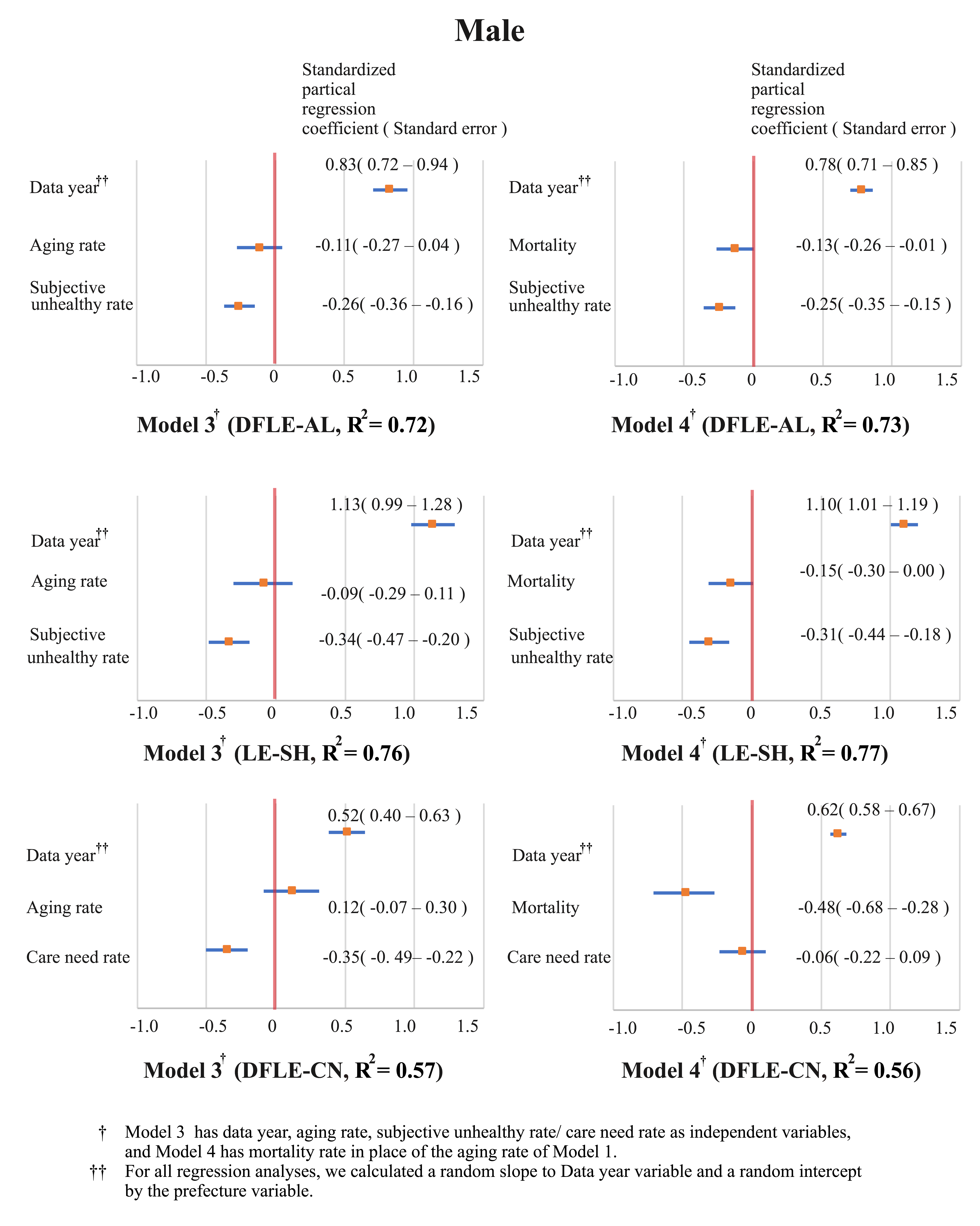
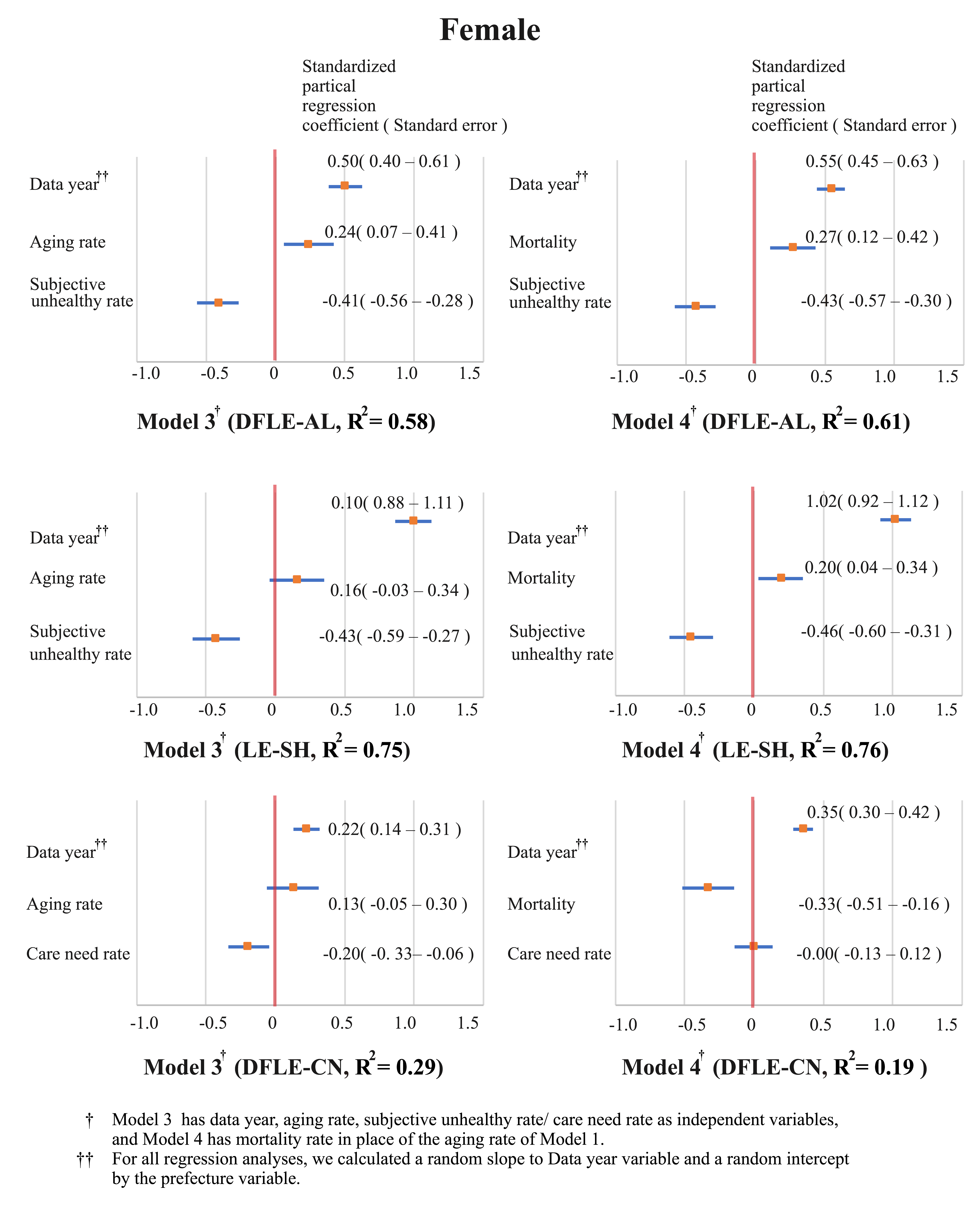
First, Cronbach’s coefficient alphas (α) for LE and the three measures of HLE were calculated to confirm their similarity. Then, regression analysis was performed using a generalized linear mixed model (GLMM), in which each HLE was used as dependent variables. Data year, aging rate, mortality, and proportion of unhealthy people were included as independent variables.
In the regression analysis, data of 47 prefectures in 2010, 2013, and 2016 were combined for all variables and treated as variables of 140 samples (the data for Kumamoto Prefecture in 2016 were missing due to an earthquake disaster). For the independent variables, the model was constructed after the evaluation of multicollinearity using a variance inflation factor (VIF). Models with both aging rate and mortality as independent variables had a high VIF value of 8.4–15.2, which could lead to multicollinearity problems. Therefore, Model 1, with data year, aging rate, restriction rate, subjective unhealthy rate, and care need rate as independent variables, and Model 2, with mortality as the independent variable in place of aging rate, were developed. In these two models, regression analyses for each HLE were performed by sex. For all regression analyses, we calculated a random slope for the data year variable and a random intercept by the prefecture variable (Figures 1 and 2).
For estimation of the parameters, simulated draws from the posterior were obtained for each parameter using the Markov chain Monte Carlo (MCMC) method.18-19 The simulated draws were preceded with 2500 “burn-in” draws, which were discarded from the analysis. The MCMC chain was thinned by including only every second draw, yielding 5000 simulated posterior observations. Then, Rhat was calculated to confirm the convergence of the simulation. Rhat is an index of the divergence between chains, and in the case of three or more chains, if it is 1.1 or less by convention, it is considered to have converged.
Analyses were performed using the open source statistical software R (ver. 3.6.2)20, and the Rstan19 package was used for parameter estimation by MCMC.