3.1 Calibration curve of arsenic
ICP-MS demonstrates ion when influencing electron multiplier especially on the dynode and it behaves as a detector. When the ions influence the dynode, there is a release of electrons and a measurable pulse is generated. Then the built-in software of ICP-MS relates the intensities and makes the calibration curve. In this study, the calibration curve was prepared for the analysis of ICP-MS to know the exact concentration of arsenic present in the solution. Linear line shows the value of R2 at 0.999 as shown in Fig.4.
3.2 Characterization of adsorbent
3.2.1 UV- Visible Spectroscopy (UV-Vis)
The absorption range of the incorporated L-cysteine derived iron oxide nanoparticle, were seen in the middle of the scope of 300-700nm wavelength. The colloidal Fe3O4 NPs were gotten and scattered in de-ionized water after the sonication process (25 minutes). Reported study, shows the fabricated NPs were in the range 375 and 650 nm [32]. In our study, the peak appeared at 394 nm of the synthesized iron oxide NPs as shown in Fig. 5.
3.2.2 Transmission Electron Microscopy (TEM)
In material sciences, TEM is used as a powerful tool for a high-resolution image. A beam of high energy of electrons moves directly towards the sample of 0.2nm. This technology investigated the shape, size and used as chemical analysis. The crystallinity, spherical morphology and size of the synthesized L-cysteine capped iron oxide NPs were analyzed as shown in Fig. 6a. The size appeared were in the range of 5-35nm and mostly were of 15nm as shown in Fig. 6b. They showed to be in a spherical shape as shown in Fig. 6a. ImageJ software was used to analyze the sizes of the particles. Yew et al. [33], observed that most particles were ranging 10-18.
3.2.3 Zeta Potential Analyzer
Zeta Potential is used to know the net surface charge of the nanoparticles and is a physical property. It also confirmed the stability of the nanoparticles concerning the surface potential charge. The stability of particles can be obtained at the most optimum line between the stable and unstable nanoparticles, which are generally expressed in the range of +30mV to -30mV. This study showed that L-cysteine capped iron oxide NPs were stable with a value of – 29.7mV as shown in Fig. 7. Madhavi et al. [34], showed that the nanoparticles were stable and contained a highly negative charge.
3.2.4 Electron Dispersion Spectrum (EDS)
EDS technique describes more about the chemical composition of the material, it also tells about the purity of the material. The spectrum at 1.73KeV at spots was examined. There were two maximum peaks of the spectrum were acquired as shown in Fig. 8. The quantitative analysis of this study revealed that there were more 68.17% weight atoms of iron are present in the synthesized Fe3O4 nanoparticles as shown in Fig. 8. Radwa et al. [35], showed that the L-cysteine is used as the stabilizing agent.
3.2.5 X-Ray Diffraction Spectroscopy
X-ray diffraction was used to determine the phase purity and the crystalline structure of the nanoparticles. The advantage of using this technique is that does not harm or damage the material and it provided results efficiently. The X-ray diffraction patters of synthesized L-cysteine capped nanoparticles showed the existence of the crystalline structure of the nanoparticles as shown in Fig. 9. The XRD peaks were matched with reported literature [36, 37]. All peaks are matched with the characteristics of magnetite material and it proposed the core-shell structure of synthesized iron oxide NPs as shown in Fig. 9.
3.2.6 Fourier Transform Infrared Spectroscopy (FT-IR)
FT-IR is a useful tool for characterizing the particles. It tells more about the capping and reduction occurring within the synthesized material. As shown in Fig. 10, the different FTIR peaks were observed. A peak at 1727cm-1 shows the presence of acidic carbonyl groups (C=O). A peak at 1083cm-1 is due to carboxyethylsilanetriol (CES) (C-O) group [38]. A peak at 1337cm-1 shows the adsorption band due to CH2 groups (bending variations). A peak at 1540cm-1 bending vibration is present [39]. A peak at 2284cm-1 shows the presence of amide groups and COO-1.
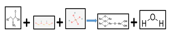
3.3 Mechanism
Arsenic creates many acute and chronic diseases in the human body. Many various technologies have been used in the past for the removal of arsenic from the water. Iron oxide adsorbents are dominant in the field of adsorption of arsenic because of its capacity. The adsorption of arsenic is mainly dependent on the quantity of iron present because iron adsorbent have the maximum ability to adsorb arsenic from the water. In our study, the L-cysteine was used as a stabilizing agent to prepare the desired particles. When the particles were fabricated it was then reacted with arsenic so that it can adsorb. After the reaction, the arsenic is reduced due to nanoparticles present in the solution. The following reaction shows how the arsenic was been adsorbed on the iron oxide nanoparticles.
3.4 Effect of adsorbent dose
The adsorption of arsenic onto the L-Cysteine functionalized Iron oxide Nanoparticles are influenced by adsorbent dose. The effect of the dose of NPs on arsenic is shown in Fig. 11. The removal percentage caused by a dose of Iron NPs of equilibrium concentrations of arsenic increases by increasing the adsorbent dose from 30 mg to 80 mg. The removal of arsenic from the aqueous solution increased from 95.4% to 99.8%. The highest removal efficiency was achieved when the maximum dose of adsorbent was added, due to the availability of maximum vacant spaces present on the surface of the adsorbent. The quantity of the adsorbent used in an experiment is directly proportional to the number of sites available for adsorption [40].
3.5 Effect of pH
The effect of pH on the adsorption is shown in Fig. 12. It is seen that the range from 5.5 to 7.5, the adsorption is higher as compared to others. At pH 6, there is maximum adsorption. The percent of removal of arsenic increases from 16% to 99.1%, as the pH increases from 4 to 8. The low adsorption rate at pH 4, which indicates that solution, becomes H+ charged and that repels the molecules of the adsorbent. Moreover, as pH rises from 4 to 8 H+ ions (positive) are replaced with OH- (negative) ions which makes arsenic molecules to attach onto the surface of the adsorbent. It is reported in the literature that the arsenic becomes unstable at higher pH [41] whereas Irem et al. [42], reported that the maximum adsorption of arsenic was on pH 6.
3.6 Effect of concentration
The effect of various concentrations on adsorption was studied using a range of arsenic concentrations from 0.01 ppm – 1 ppm (10 ppb – 1000ppb) at a fixed adsorbent dose of 80 mg, using an orbital shaker speed of 150 rpm at room temperature. The batch study is shown in Fig. 13. The results depict that there was a maximum removal in the lowest concentration at 0.01 ppm (10 ppb) was 99.85% and the minimum removal was observed in the highest concentration at 1 ppm (1000 ppb) was 94.45% as shown in Fig. 14. Even at 0.5ppm (500ppb), the removal efficiency was 98.9% after one hour.
3.7 Equilibrium isotherms
For to understand the functioning of adsorbing molecule and adsorbent for the optimization process design [43]. From the experimental data, the values were put into two isotherm models. Isotherm parameters for each model was obtained from intercept and slope of model equation.
3.7.1 Langmuir Isotherm Model
The Langmuir isotherm model believes that the adsorption happens at certain equivalent destinations inside the adsorbent. The monolayer adsorption venture is shown as [44].
In Langmuir model, the adsorption
Ce/qe = 1/Qmax * KL + Ce/Qmax -------------- (3)
Where,
Ce = concentration of arsenic at equilibrium (mg/l)
qe = equilibrium capacity of arsenic on the adsorbent (mg/g)
Qmax = monolayer adsorption capacity (mg/g)
KL = Langmuir adsorption constant (L/mg)
The values Qmax and KL can be calculated from the slope and the intercept of the linear plot shown in Fig. 14. The value and constant of R2 from the equilibrium data shown in Table 2. The important characteristic of the Langmuir isotherm can be demonstrated as the dimensionless constant separation factor RL which is shown by this equation
The significant normal for the Langmuir isotherm can be exhibited as the dimensionless constant factor RL which is appeared by this condition [45].
RL = 1/(KL+Co) ---------- (4)
Where,
Co = Initial concentration (mg/l)
KL = Langmuir constant (l/mg)
In the Freundlich isotherm, surface adsorption occurs in multilayer or heterogeneous [46]. The Freundlich equation is follow as [47];
log qe = log KF + 1/n *(log Ce) ------------- (5)
where,
qe = amount of solute adsorbed per unit weight of adsorbent (mg/g)
Ce = equilibrium concentration (mg/L)
KF = Freundlich constant indication to the relative adsorption capacity of the adsorbent (mg/g)
1/n is the adsorption intensity.
The values of KF and 1/n will be obtained from the linear plot of log qe versus log Ce shown in Fig. 15. The isotherm parameters and R2 value are presented in Table 4.1.
In this isotherm study, it was well concluded that the Langmuir isotherm fitted the best for the synthesized nanoparticles as shown in Fig. 14. The maximum adsorption capacity was calculated to be 1.96 mg/g. The parameters of both the models, Langmuir and Freundlich are mentioned in Table 2. The values are being checked by different researches and they used three isotherm models [48, 49], whereas this study performed only two isotherm models.
3.8 Kinetic study
For the determination of efficiency of adsorbent in relation of solute consuming rate which can be described by adsorption kinetics. Therefore, the experimental data was shown through pseudo first-order, pseudo second-order to describe the mass transfer process.
3.8.1 Pseudo-first-order model
The Pseudo first-order equation [50] can be expressed as:
ln (qe – qt) = ln qe - k1* t ---------- (6)
Where,
qe = amount of arsenic adsorbed at equilibrium (mg/g)
qt = amount of arsenic adsorbed at time t (mg/g)
k1 = pseudo first order rate constant
The value of k1 and qe can be calculated from slope and intercept by plotting graph between, ln (qe – qt) versus t as shown in Fig. 16, and the values of constants are presented in Table 3.
3.8.2 Pseudo-second-order model
The pseudo second-order model can be expressed as [51];
t/qt = k2q2e + t/qe ------------ (7)
where,
k2 = a second-order rate equation constant and can be obtained by plotting the graph t/qe versus t, shown in Fig. 17, and the calculated values of constants are shown in Table 3.
In the current study, the kinetics of arsenic removal was studied to find and to know the adsorption capacity and adsorption behavior. Adsorption increased with the passage of time as there are vacant spaces available on the adsorbent but after the equilibrium achieved the adsorption starts to decrease and become resistant as the vacant site are occupied. This work followed Pseudo 2nd order and confirms the chemical adsorption as shown in Fig. 18, whereas, Pseudo 1st order confirms physical adsorption. Rahdar et al. [50] also performed the datasets into the kinetic study i.e., two models. In this study, Pseudo 2nd order fitted the best. The values for both kinetic orders are mentioned in Table 3.
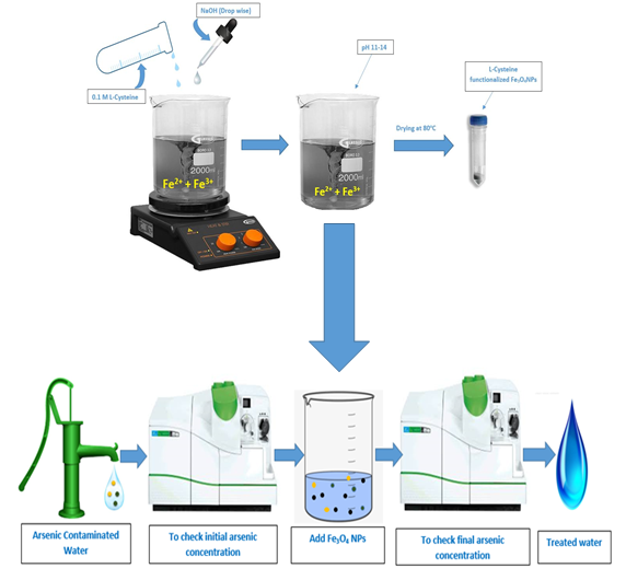
3.9 Testing of real water samples
As discussed in methodology part, three areas were select for the site selection, sample preparation and analysis on ICP-MS of real water. The basic physical and chemical parameters of water samples as shown in Table 4.
After testing the basic parameters, we then tested arsenic presence by the arsenic kit. It confirmed the arsenic presence in the water and after then the samples were collected. Those samples were than tested on ICP-MS for further confirmation and to know the initial reading, after knowing the initial arsenic level 80mg of iron oxide NPs, were added and kept on stirrer for 30 and 60 min as shown in Fig.18.
Fluoride was also tested through spectrophotometer (DR-1900) but none of the sample had more fluoride than the permissible limit. The permissible limit of fluoride by WHO was reported at 1.5 ppm. In Table 5, it can be seen that the maximum removal after 30 minutes was 77.3% and when it kept for 60 minutes, the maximum adsorbed efficiency was 81.09%. Table 6 shows the comparison data of the reported and this present study.