We compared the features of participants who chose “Accept” and “Not now” as their final decision in MEG. We found that participants who chose “Accept” had higher scores than those who chose “Not now” for KnowPSA (2.23 ± 0.81 vs 2.07 ± 0.69, p = 0.002), IPSS1 (1.31 ± 1.48 vs 0.70 ± 1.06, p < 0.000), IPSS2 (1.33 ± 1.42 vs 0.74 ± 1.09, p < 0.000), IPSS3 (1.20 ± 1.53 vs 0.64 ± 1.10, p = 0.008), IPSS4 (1.15 ± 1.46 vs 0.66 ± 1.08, p = 0.025), IPSS5 (0.87 ± 1.26 vs 0.42 ± 0.89, p = 0.003), and IPSS7 (2.02 ± 1.29 vs 1.60 ± 1.10, p = 0.045). This finding suggests that participants with higher IPSS score tended to choose “Accept” for PSA screening as their decision. Regarding IPPI items, participants who chose “Accept” scored high in A (3.93 ± 1.07 vs 3.20 ± 1.29, p < 0.000), B (3.60 ± 1.26 vs 3.26 ± 1.37, p < 0.000), C (3.88 ± 1.15 vs 3.60 ± 1.17, p = 0.006), D (3.42 ± 1.35 vs 3.05 ± 1.59, p = 0.001), E (4.43 ± 0.85 vs 3.31 ± 1.26, p < 0.000), F (4.16 ± 1.00 vs 2.96 ± 1.49, p < 0.000), H (2.94 ± 1.26 vs 2.84 ± 1.67, p = 0.004), I (3.71 ± 1.25 vs 3.47 ± 1.44, p = 0.005), J (3.43 ± 1.29 vs 3.01 ± 1.63, p < 0.000). This notably demonstrated that participants who care about physiological and psychological impacts more were more likely to choose “Accept”. By contrast, subjects who did not care about the positive and negative impact of PSA screening were less likely to receive PSA screening. Age, RiskUThink, IPSS6, and item G of IPPI were similar for both groups (Table 1a).
Participants who chose “Not now” were more likely to be widowed or have a low education level. Important priorities were significantly different between participants who chose “Accept” and those who chose “Not now” (Table 1b). Logistic regression showed that KnowPSA; IPSS7; and IPPI A, D, F, G, J, first and second concerns were statistically significant predictors of the final decision. KnowPSA (odds ratio [OR]: 0.539, CI: 0.336–0.865, p = 0.010), IPSS7 (OR: 0.612, CI: 0.432–0.868, p = 0.006), A (OR: 0.663, CI: 0.474–0.928, p = 0.017), D (OR: 0.623, CI: 0.434–0.895, p = 0.010), F (OR: 0.532, CI: 0.350–0.807, p = 0.003), J (OR: 0.686, CI: 0.473–0.996, p = 0.048) were negative predictors for the “Not now” decision, whereas G (OR: 1.452, CI: 1.028–2.049, p = 0.034) was the positive predictor for the same. Regarding the first concern, the answers “A”, “B”, “D”, and “J” were positively associated with “Not now” with “I” as the reference category. For the second concern, the answer “A” was positively associated with “Not now” with “C” as the reference category (Table 1a, 1b).
Table 1
a. Comparison of features of participants in the MEG with their final decisions of “Accept” and “Not now”; continuous and ordinal variables
| Features | Model Establish Group (N = 507) |
| Univariate analysis | Multivariate analysis |
| "Accept" (N = 130) | "Not Now" (N = 377) | All (N = 507) | | Logistic regression (“Accept”:0;“Not now”:1) |
| Mean ± SD | Mean ± SD | Mean ± SD | P value | Coefficient | SE | Odds Ratio (95% CI) | P value |
| Age(y/o) | 63.63 ± 9.41 | 62.63 ± 9.80 | 62.89 ± 9.70 | 0.335 | 0.018 | 0.021 | 1.018 (0.977, 1.061) | 0.397 |
| KnowPSA1 | 2.23 ± 0.81 | 2.07 ± 0.69 | 2.11 ± 0.73 | 0.002* | -0.619 | 0.241 | 0.539 (0.336, 0.865) | 0.010* |
| RiskUThink2 | 2.61 ± 1.12 | 2.47 ± 1.02 | 2.50 ± 1.05 | 0.897 | -0.149 | 0.170 | 0.861(0.617,1.202) | 0.380 |
| IPSS | IPSS 1 | 1.31 ± 1.48 | 0.70 ± 1.06 | 0.86 ± 1.21 | 0.000* | -0.117 | 0.193 | 0.890(0.610,1.299) | 0.545 |
| IPSS 2 | 1.33 ± 1.42 | 0.74 ± 1.09 | 0.89 ± 1.21 | 0.000* | 0.003 | 0.203 | 1.003(0.674,1.495) | 0.986 |
| IPSS 3 | 1.20 ± 1.53 | 0.64 ± 1.10 | 0.78 ± 1.25 | 0.008* | -0.258 | 0.214 | 0.772(0.507,1.175) | 0.228 |
| IPSS 4 | 1.15 ± 1.46 | 0.66 ± 1.08 | 0.78 ± 1.21 | 0.025* | -0.156 | 0.224 | 0.856(0.551,1.328) | 0.487 |
| IPSS 5 | 0.87 ± 1.26 | 0.42 ± 0.89 | 0.53 ± 1.02 | 0.003* | -0.232 | 0.237 | 0.793(0.499,1.262) | 0.328 |
| IPSS 6 | 0.81 ± 1.28 | 0.58 ± 1.02 | 0.64 ± 1.10 | 0.518 | 0.372 | 0.210 | 1.451(0.961,2.190) | 0.077 |
| IPSS 7 | 2.02 ± 1.29 | 1.60 ± 1.10 | 1.71 ± 1.16 | 0.045* | -0.490 | 0.178 | 0.612(0.432,0.868) | 0.006* |
| IPSS Q3 | 4.85 ± 1.45 | 5.21 ± 1.28 | 5.12 ± 1.33 | 0.169 | -0.088 | 0.220 | 0.916(0.595,1.409) | 0.690 |
| IPPI | A | 3.93 ± 1.07 | 3.20 ± 1.29 | 3.39 ± 1.27 | 0.000* | -0.411 | 0.172 | 0.663(0.474,0.928) | 0.017* |
| B | 3.60 ± 1.26 | 3.26 ± 1.37 | 3.35 ± 1.35 | 0.000* | -0.105 | 0.180 | 0.901(0.633,1.282) | 0.562 |
| C | 3.88 ± 1.15 | 3.60 ± 1.17 | 3.67 ± 1.17 | 0.006* | 0.339 | 0.218 | 1.403(0.915,2.153) | 0.121 |
| D | 3.42 ± 1.35 | 3.05 ± 1.59 | 3.14 ± 1.54 | 0.001* | -0.473 | 0.185 | 0.623(0.434,0.895) | 0.010* |
| E | 4.43 ± 0.85 | 3.31 ± 1.26 | 3.60 ± 1.26 | 0.000* | -0.441 | 0.246 | 0.644(0.397,1.043) | 0.073 |
| F | 4.16 ± 1.00 | 2.96 ± 1.49 | 3.27 ± 1.48 | 0.000* | -0.632 | 0.213 | 0.532(0.3500.807) | 0.003* |
| G | 2.29 ± 1.37 | 2.25 ± 1.62 | 2.26 ± 1.56 | 0.341 | 0.373 | 0.176 | 1.452(1.0282.049) | 0.034* |
| H | 2.94 ± 1.26 | 2.84 ± 1.67 | 2.86 ± 1.57 | 0.004* | 0.312 | 0.207 | 1.366(0.9112.048) | 0.132 |
| I | 3.71 ± 1.25 | 3.47 ± 1.44 | 3.53 ± 1.40 | 0.005* | 0.075 | 0.190 | 1.078(0.7431.564) | 0.692 |
| J | 3.43 ± 1.29 | 3.01 ± 1.63 | 3.12 ± 1.56 | 0.000* | -0.377 | 0.190 | 0.686(0.4730.996) | 0.048* |
Table 1
b. Comparison of features in MEG subjects between “Accept” and “Not now”; categorical variables
| Features (reference) | Model Establish Group (N = 507) |
| Univariate analysis | Multivariate analysis |
| | Final decision | χ2 | Logistic regression (“Accept”:0,“Not now”:1) |
| | "Accept" (N = 130)" | Not Now" (N = 377) | P value | Coefficient | SE | Odds Ratio (95% CI) | P value |
| Marriage4 (Married) | | | | 0.000 | | | | 0.145 |
| Divorce | 5(3.8) | 0(0) | -24.02 | 15358 | 0.00 (0.00) | 0.999 |
| Single | 9(6.9) | 9(2.4) | -1.508 | 0.747 | 0.221 (0.051,0.957) | 0.043* |
| Widow | 6(4.6) | 31(8.2) | 0.834 | 0.698 | 2.304 (0.587,9.045) | 0.232 |
| Education5 (> 12 years) | | | | 0.079 | | | | 0.674 |
| <=9 years | 61(46.9) | 195(51.7) | 0.130 | 0.423 | 1.139 (0.497,2.608) | 0.759 |
| > 9,<=12 years | 34(26.2) | 115(30.5) | 0.375 | 0.433 | 1.455 (0.623,3.399) | 0.387 |
| PcaFriend6(Yes) | No | 34(26.2) | 69(18.3) | 0.038 | -0.005 | 0.423 | 0.995 (0.434,2.280) | 0.990 |
| The 1st concern(I)7 Omit insignificant | I | 25(19.2) | 79(21.0) | 0.000 | | | | 0.003* |
| A | 32(24.6) | 56(14.9) | 2.133 | 0.664 | 8.442 (2.298,31.017) | 0.001* |
| B | 10(7.7) | 75(19.9) | 1.641 | 0.716 | 5.161 (1.267,21.017) | 0.022* |
| D | 3(2.3) | 39(10.3) | 3.779 | 1.026 | 43.765(5.856,327.091) | 0.000* |
| J | 4(3.1) | 25(6.6) | 2.164 | 0.918 | 8.704 (1.440,52.613) | 0.018* |
| The 2nd concern(C)8 Omit insignificant | C | 18(13.8) | 69(18.3) | 0.000 | | | | 0.005* |
| A | 5(3.8) | 24(6.4) | 2.394 | 0.991 | 10.958(1.571,76.422) | 0.016* |
| The 3rd concern(C)9 Omit insignificant | C | 28(21.5) | 84(22.2) | 0.000 | | | | 0.227 |
| J | 9(6.9) | 56(14.9) | 1.797 | 0.798 | 6.029(1.261,28.831) | 0.024* |
| *: statistically significant, Mann–Whitney U Test for continuous and ordinal variables; χ2 test for categorical variables. |
| 1. KnowPSA: item that measures previous knowledge about PSA (Score 1: Not heard, Score 2: Little, Score 3: Much). |
-
2. RiskUThink: item that measures the degree of perception of risk for prostate cancer. How much risk of prostate cancer do you have? (1: Rare, 2: Little, 3: Same as others, 4: Much, 5: Very likely).
-
3. IPSSQ: the quality of life item in the IPSS.
-
4. Marriage status includes D: divorced, M: married, S: single, and W: widow.
-
5. Education status was divided into J: diploma less than or equal to junior high school graduation, S: diploma above junior high school, but less than or equal to senior high school graduation, U: diploma above senior high school graduation.
-
6. PcaFriend: Do you have any friend or relative who has been diagnosed with prostate cancer? Y: yes, N: no.
-
7. First: From items A to J in the IPPI, which one is the most important factor that influences your decision?
-
8. Second: From items A to J in the IPPI, which one is the second most important factor that influences your decision?
-
9. Third: From items A to J in IPPI, which one is the third most important factor that influences your decision?
A: Physiological impact: life prolongation resulting from the PSA blood test.
B: Physiological impact: side effects of unnecessary repeated biopsy resulting from false-positive PSA blood tests.
C: Physiological impact: chance of loss of survival time resulting from false-negative blood tests.
D: Physiological impact: side effects of receiving unnecessary definite treatment for insignificant prostate cancer discovered by a PSA blood test.
E: Psychological impact: being satisfied by PSA test in knowing my health conditions.
F: Psychological impact: Feeling easy resulting from normal results of PSA test.
G: Psychological impact: being tense before PSA blood test.
H: Psychological impact: being anxious after getting abnormal PSA test results.
I: Psychological impact: the psychological impact of being misdiagnosed as normal by PSA test.
J: Psychological impact: being severely anxious after knowing the diagnosis of prostate cancer discovered by PSA test.
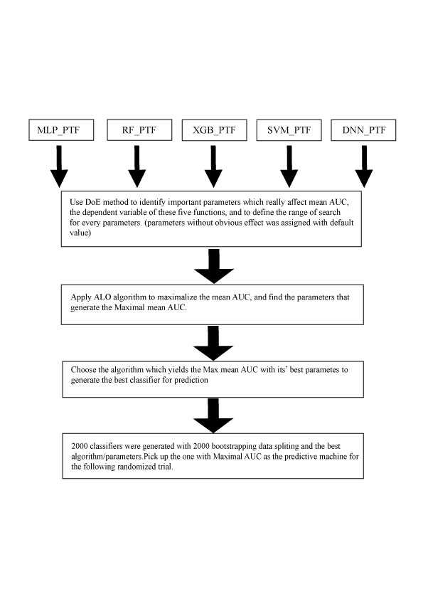
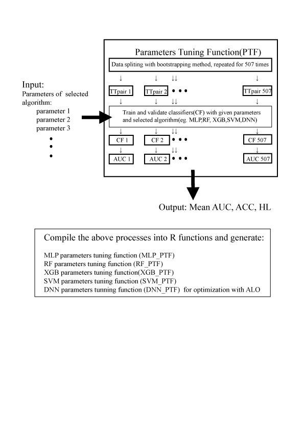
The accuracy and AUC of models constructed using the MEG dataset were calculated to find the model with the best performance. Initially, we performed a logistic regression using the same unbiased data-splitting method [45]. We obtained the mean accuracy (0.8140), the highest accuracy among LR models (0.8763), the mean AUC (0.7947), and the highest AUC among LR models (0.8939). Obviously, the DoE–ALO parameter tuning method is not suitable in logistic regression. In terms of machine-learning models, we found the best parameters for all five machine-learning algorithms (Supplement 4). We observed the DNN and RF models to have the highest mean accuracy (0.8429, 0.8313) after parameter tuning. The pairwise comparison showed no significant differences in the accuracy between DNN and MLP models. Moreover, RF models have the highest mean AUC (0.8801) after parameter tuning. Because our MEG dataset is relatively imbalanced, the AUC would be better than accuracy as a performance measurement according to a study published by Charles et al. [50]. Accordingly, we chose the model with the best mean AUC, that is the RF model, as the decision-suggesting tool in our study (Fig. 2). The accuracy of the best model with the best parameters among the models constructed using 2000 iterations of bootstrapping is 0.9000. Thus, the RF model was used to build the user interface for the RCT.
We randomized participants into the MLSG and CG. In total, 380 participants accomplished all steps of the experiment. Five of the MLSG and eight of the CG were dropped because of poor answer quality which we mentioned earlier in the Methods section. There was no important harms or unintended effects in each group. The participants of both groups showed similarity in age, KnowPSA, RiskUThink, IPSS1-3, IPS5-7, IPSS Q, and all items of IPPI. The participants in the MLSG had significantly higher IPSS4 scores than those in the CG. They also scored higher than the participants of the CG in A (3.26 ± 1.466 vs 3.04 ± 1.221), H (2.28 ± 1.933 vs 1.92 ± 1.757), I (2.86 ± 1.641 vs 2.58 ± 1.446) although it did not reach the significance level. The participants of MLSG and CG also showed similarity in marriage status, education level, PcaFriend, and priorities of the importance of impact items (Supplement 5).
Regarding SSTI items, we found that participants in the MLSG were calmer (SSTI1: 2.28 ± 1.210 vs 1.98 ± 1.142, p = 0.004), more content (SSTI5: 2.12 ± 1.219 vs 1.87 ± 1.108, p = 0.031), and less worrisome (SSTI6: 2.00 ± 1.022 vs 2.98 ± 1.166, p < 0.000) than those in the in CG. They also experienced higher satisfaction than those in the CG toward the decision-making process, including more adequately informed (Sa1: 1.75 ± 0.928 vs 3.21 ± 1.560, p < 0.000), assurance that the decision is the best one (Sa2: 1.83 ± 0.886 vs 3.29 ± 1.440, p < 0.000), consistency with personal values (Sa3: 1.77 ± 0.894 vs 3.19 ± 1.605, p < 0.000), willing to carry out the decision (Sa4: 1.67 ± 0.824 vs 3.13 ± 1.698, p < 0.000), and satisfaction (Sap: 1.57 ± 0.818 vs 3.12 ± 1.674, p < 0.000). The DCS is a five-scale questionnaire with a reverse scoring system, that is, strongly agree: score 0 and strongly disagree: score 5. We found that the participants in the MLSG perceived that they had more decision support (DCS7: 1.85 ± 1.052 vs 2.19 ± 1.244, p = 0.012), decision advice (DCS9: 1.73 ± 0.951 vs 2.30 ± 1.175, p < 0.000), assurance of the decision (DCS10: 1.88 ± 0.993 vs 2.26 ± 1.264, p = 0.008; DCS11: 1.81 ± 0.981 vs 2.38 ± 1.228, p < 0.000), ease of decision-making (DCS12: 1.81 ± 0.939 vs 2.43 ± 1.232, p < 0.000), adherence to the decision (DCS15: 1.78 ± 0.872 vs 2.08 ± 1.168, p = 0.040), and more satisfaction (DCS16: 1.60 ± 0.739 vs 1.98 ± 1.092, p = 0.004; Table 2).
Table 2
Comparison of SSTI, satisfaction, and DCS between MLSG and CG
| Features | MLSG vs CG (N = 367) |
| MLSG (N = 185) | "CG" (N = 182) | All (N = 367) | p value |
| Mean | SD | Mean | SD | Mean | SD | |
| Anxiety | SSTI1 | 2.28 | 1.210 | 1.98 | 1.142 | 2.13 | 1.185 | 0.004* |
| SSTI2 | 2.22 | 0.987 | 2.08 | 0.901 | 2.15 | 0.947 | 0.146 |
| SSTI3 | 2.21 | 1.090 | 2.36 | 1.051 | 2.29 | 1.072 | 0.176 |
| SSTI4 | 2.15 | 1.197 | 1.97 | 1.132 | 2.06 | 1.167 | 0.069 |
| SSTI5 | 2.12 | 1.219 | 1.87 | 1.108 | 2.00 | 1.170 | 0.031* |
| SSTI6 | 2.00 | 1.022 | 2.98 | 1.166 | 2.49 | 1.198 | 0.000* |
| Decision Satisfactory | Sa1 | 1.75 | 0.928 | 3.21 | 1.560 | 2.48 | 1.474 | 0.000* |
| Sa2 | 1.83 | 0.886 | 3.29 | 1.440 | 2.55 | 1.399 | 0.000* |
| Sa3 | 1.77 | 0.894 | 3.19 | 1.605 | 2.47 | 1.478 | 0.000* |
| Sa4 | 1.67 | 0.824 | 3.13 | 1.698 | 2.39 | 1.516 | 0.000* |
| Sa5 | 1.57 | 0.818 | 3.12 | 1.674 | 2.34 | 1.524 | 0.000* |
| Decision Conflicts | DCS1 | 2.09 | 0.965 | 2.29 | 1.115 | 2.19 | 1.045 | 0.143 |
| DCS2 | 2.23 | 1.028 | 2.18 | 1.157 | 2.20 | 1.093 | 0.321 |
| DCS3 | 2.24 | 1.097 | 2.19 | 1.098 | 2.22 | 1.096 | 0.658 |
| DCS4 | 2.23 | 1.095 | 2.16 | 1.187 | 2.20 | 1.140 | 0.377 |
| DCS5 | 2.17 | 1.088 | 2.33 | 1.244 | 2.25 | 1.169 | 0.329 |
| DCS6 | 2.29 | 1.089 | 2.42 | 1.254 | 2.36 | 1.174 | 0.438 |
| DCS7 | 1.85 | 1.052 | 2.19 | 1.244 | 2.02 | 1.163 | 0.012* |
| DCS8 | 2.05 | 1.178 | 1.91 | 1.060 | 1.98 | 1.122 | 0.311 |
| DCS9 | 1.73 | 0.951 | 2.30 | 1.175 | 2.01 | 1.104 | 0.000* |
| DCS10 | 1.88 | 0.993 | 2.26 | 1.264 | 2.07 | 1.150 | 0.008* |
| DCS11 | 1.81 | 0.981 | 2.38 | 1.228 | 2.09 | 1.146 | 0.000* |
| DCS12 | 1.81 | 0.939 | 2.43 | 1.232 | 2.12 | 1.136 | 0.000* |
| DCS13 | 1.89 | 1.053 | 2.12 | 1.178 | 2.01 | 1.121 | 0.076 |
| DCS14 | 1.96 | 0.952 | 2.15 | 1.061 | 2.06 | 1.011 | 0.108 |
| DCS15 | 1.78 | 0.872 | 2.08 | 1.168 | 1.93 | 1.039 | 0.040* |
| DCS16 | 1.60 | 0.739 | 1.98 | 1.092 | 1.79 | 0.949 | 0.004* |
| *: statistically significant, Mann–Whitney U Test was used. |
We also wondered about the influence of machine-learning suggestions on the final decisions of participants. We observed that 24.18% of participants in the CG chose “Accept”, whereas 75.82% chose “Not now” as their final decision. Participants who were suggested to “Accept” by the machine-learning model had a higher chance of making “Accept” their final decision than those in CG deciding on “Accept” (50.75% vs 24.18%, χ2 = 16.07, p < 0.000). Similarly, participants who were suggested “Not now” tended to be more likely to make it their final decision, even though it was statistically insignificant (75.82% vs 82.20%, χ2 = 1.72, p = 0.190; Table 3).
Table 3
Effects of machine-learning suggestions on final decision
| | | Final Decision | |
| | | “Accept”(%) | “Not now”(%) | Sum | Chi-square, p-value, |
| MLSG | Suggest”Accept” | 34(50.75) | 33(49.25) | 67 | χ2 = 16.07, p < 0.000* |
| CG | No suggestion | 44(24.18) | 138(75.82) | 182 | |
| | Sum | 78 | 171 | 249 | |
3a. Comparison of final decision between participants who got suggestion of “Accept” and those who got no suggestions in the CG
| | | Final Decision | |
| | | “Accept”(%) | “Not now”(%) | Sum | Chi-square, p-value, |
| MLSG | Suggest”Not now” | 21(17.80) | 97(82.20) | 118 | χ2 = 16.07, p < 0.000* |
| CG | No suggestion | 44(24.18) | 138(75.82) | 182 | |
| | Sum | 65 | 235 | 300 | |
| 3b.Comparison of final decision between subjects got suggestion of “Not now” and those who got no suggestions in the CG |