Experimental design
Data from the NCORE project was used in this work. NCORE employed fMRI to characterise whether aprepitant (a neurokinin-1 receptor antagonist) modulated the neural correlates of reward processing, emotional processing, and cue reactivity in people with moderate-severe sOUD receiving methadone (MD) in comparison with HC. Only data from the placebo scanning session was used in these analyses described below. A detailed description of the study design can be found elsewhere13, and a description of the MID and Cue Reactivity tasks can be found in Supplementary Materials, Methods.
Participants
MD participants (n = 29) were recruited from community-based NHS and/or voluntary sector run drug and alcohol services based in London and surrounding areas. Potential participants were identified by via investigator led caseload screening, direct keyworker/clinician referral, or advertisement at services. Healthy volunteers (n = 22) were recruited via advertisement in press, on social media, volunteer databases or poster advertisements.
Inclusion criteria for all participants were as follows: (i) aged over 18 years; (ii) males or females. Exclusion criteria for all participants included: (i) intoxication at any of the screening or study visits; (ii) positive drug (except for cannabis) and alcohol screens at any of the screening or study visits; (iii) the use of regular relapse prevention medications; (iv) any physical or mental health issues that may affect study safety or integrity; (v) any MRI contraindication.
Main inclusion criteria for MD individuals included: (i) DSM-5 diagnosis of current, severe sOUD; (ii) currently treated with methadone substitution therapy (< 60mgs/day) and able to maintain the same dose across two scanning sessions separated by at least five days. Main exclusion criteria for MD participants included: (i) current alcohol or substance use disorder apart from opioid or nicotine; (ii) current severe DSM-5 mental health disorder; (iii) regular on-top use of heroin, opiates or other illicit substances except cannabis.
Main exclusion criteria for HC included: (i) current or history of substance or alcohol use disorder apart from nicotine; (ii) current or history of pathological gambling; (iii) current DSM-5 psychiatric disorder; (iv) current regular use of psychotropic medication that cannot be paused for the duration of the study.
The study was approved by the West London & GTAC ethics committee (REC:19/LO/0971) and performed in accordance with the principles of the Declaration of Helsinki. All participants provided written informed consent.
Preprocessing
Preprocessing was conducted using the fMRI Expert Analysis Tool (FEAT, Version 6.00) from the FMRIB Software Library (FSL)18,19. Preprocessing consisted of interleaved slice-time correction, brain extraction using FSL’s Brain Extraction Tool (BET), motion correction in 6 degrees of freedom with FSL’s MCFLIRT, and spatial smoothing with a 5mm at full-width at half maximum Gaussian kernel filter. Framewise Displacement was computed as metric of motion artefact. Subject-level Independent Component Analysis (ICA) was conducted with FSL’s ICA AROMA algorithm20, which classified each of the data-driven number of components as either signal or noise. Components identified as noise were regressed out using FSL’s regfilt function.
Mutual information functional connectivity (miFC)
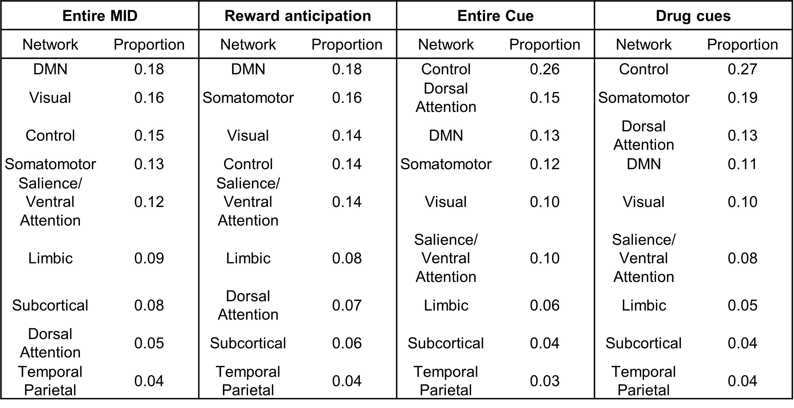
We used mutual information as a nonparametric assessment of dependence between two signals21–24. Cortical regions were defined using the 200-parcel, 17-network Shaefer atlas25,26 was registered to subject space. Subcortical regions were identified using Freesurfer’s recon_all function27. The remaining steps to compute pairwise miFC were conducted in line with our previous work28. Timeseries were extracted from each region and z-scored to centre mean 0 and ± 1 standard deviation. Algorithms to compute pairwise miFC29 generated a symmetric 214-by-214 miFC matrix (Fig. 1Ai).
To compute miFC during the conditions of interest, explanatory variables were used to create a “task timeseries” for each participant (Fig. 1Aii). The task timeseries was convolved with a canonical haemodynamic response function using SPM and identified volumes acquired during the conditions of interest for each task. The condition of interest for the MID task was reward anticipation, whereas for the Cue Reactivity it was blocks of drug-related cues. These volumes were concatenated, thus generating a “timeseries” solely during the condition of interest. The remaining miFC computation and statistical analysis was conducted in line with that performed on the entire task timeseries.
µ-Opioid Receptor and DRD2 Availability
Positron Emission Tomography (PET) images were sourced from a study that collated PET images from 26 studies to create a normative atlas of 19 different receptors, including MOR and DRD2s17.
The MOR availability image was created using two studies, of which we only used one30. The study by Kantonen et al was included for its large sample size (n = 204), and the other study included participants from the study by Kantonen in their cohort, rendering the PET images non-independent31. In line with Hansen et al, an average DRD2 image was created from the mean of three studies32–34
The PET images were already parcellated into the same 200 cortical regions used in this work. To obtain the receptor availability for the subcortical regions included in this work, masks of subcortical regions were used to extract receptor availability from the volumetric PET images, which were added to the cortical parcellations. Then, as in Hansen et al, the receptor densities were z-scored across all regions to centre mean 0 with ± 1 standard deviation. To increase the interpretability of computing the pairwise sum of receptor densities, the z-scored receptor densities were rescaled between 0 and 1.
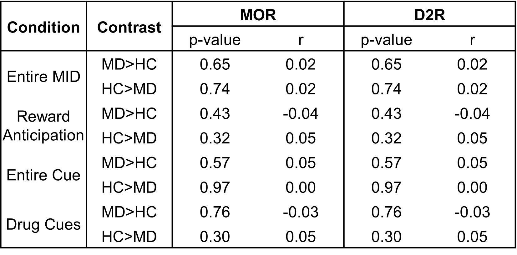
The pairwise sum of receptor densities was computed to assess the relationship between receptor densities and the z-stat for significant group differences in miFC (Fig. 1B). Considering that the sum of receptor availability could result from either two regions with equivalent receptor densities, or one region with high and one with low receptor availability, we also assessed the relationship between the miFC results and the ratio of receptor availability between each pair of regions. We show that the results presented for the pairwise sum were not replicated when using the ratio of receptor availability (Supp Mat Table 1).
Defining brain states
Regional BOLD signal timeseries were demeaned, band-pass filtered by a 2nd order Butterworth filter (passband of 0.02–0.1 Hz), then Hilbert transformed to an analytic signal as in Eq. 1:
$$X\left(t\right)=A\left(t\right)\text{cos}\left(\theta \left(t\right)\right),$$
1
where A(t) is the instantaneous amplitude, and θ(t) is the instantaneous phase. The phase angle was used to compute a FC matrix as in Eq. 2:
$$FC\left(n,p,t\right)=\text{cos}\left(\theta \left(n,t\right)\right)-\theta (p,t))$$
2
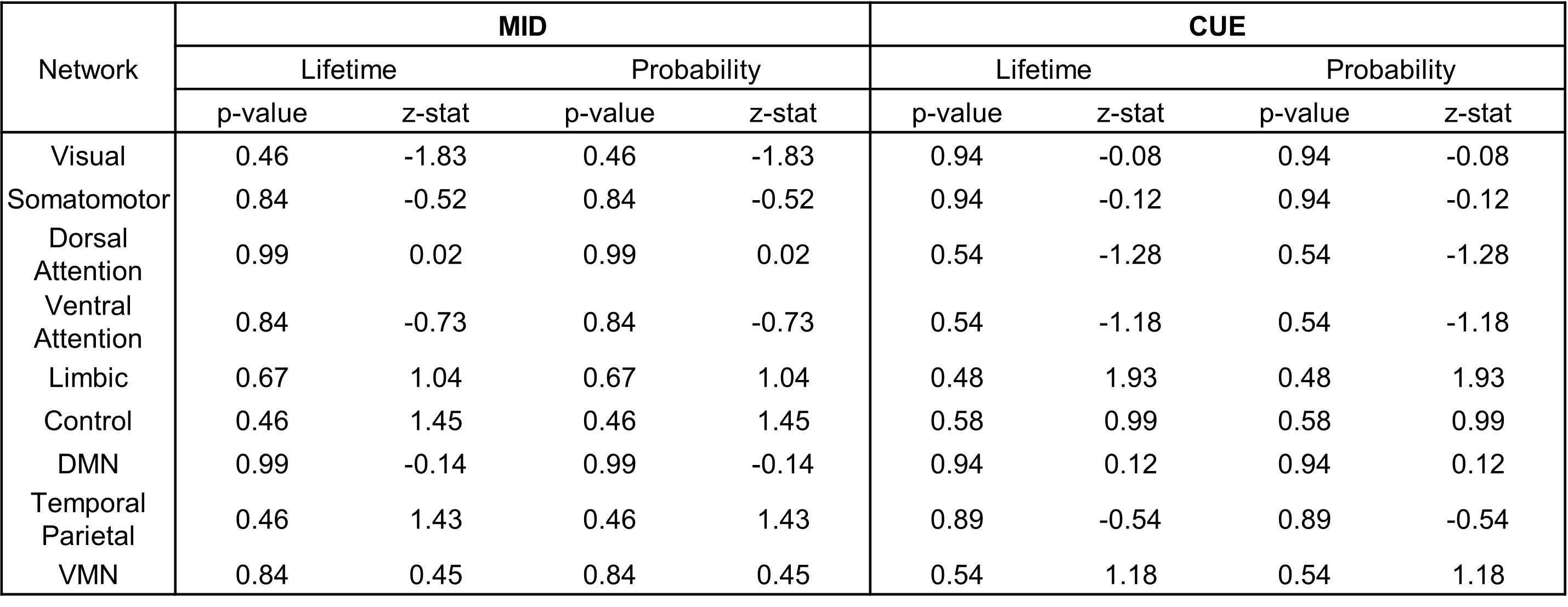
where FC(n,p,t) contains the phase coherence between brain areas n and p at time t. FC(n,p,t) was masked by binary matrices representing each of the eight canonical functional networks26 and the VMN12. The mean coherence across all regions included in each of the template networks was computed from the upper triangle of FC(n,p,t) with the diagonal omitted. Timepoint t was assigned the network with highest average coherence, generating a state timeseries (Fig. 1C).
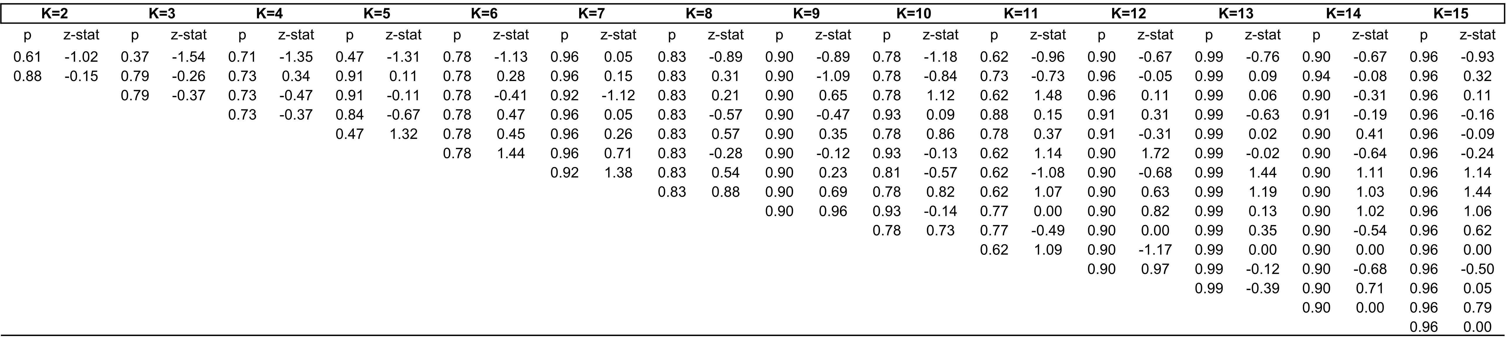
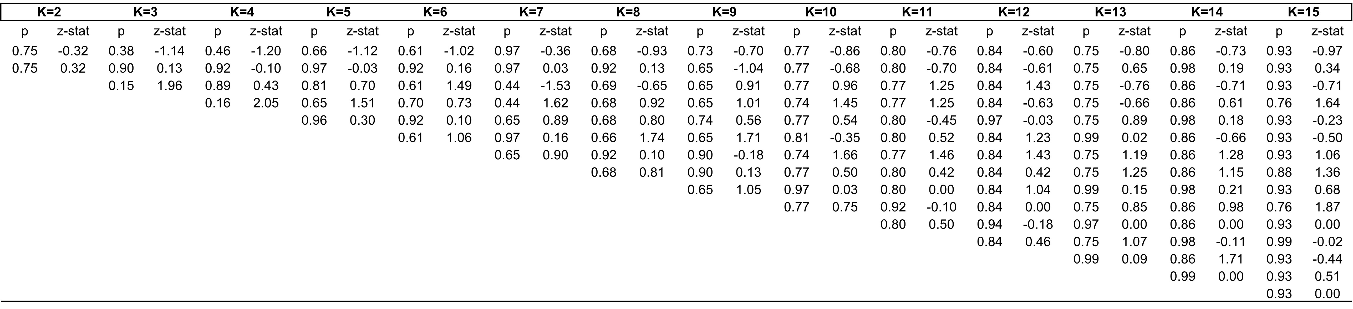
To ensure dynamical FC results are not a by-product of this unique method, we also computed brain states and state timeseries using a conventional dynamical FC analysis35,36. The results of analyses assessing the effect of group on metrics of brain state dynamics replicate those presented in the Results section (Supp Mat Methods and Tables 2–7).
Metrics of brain state dynamics
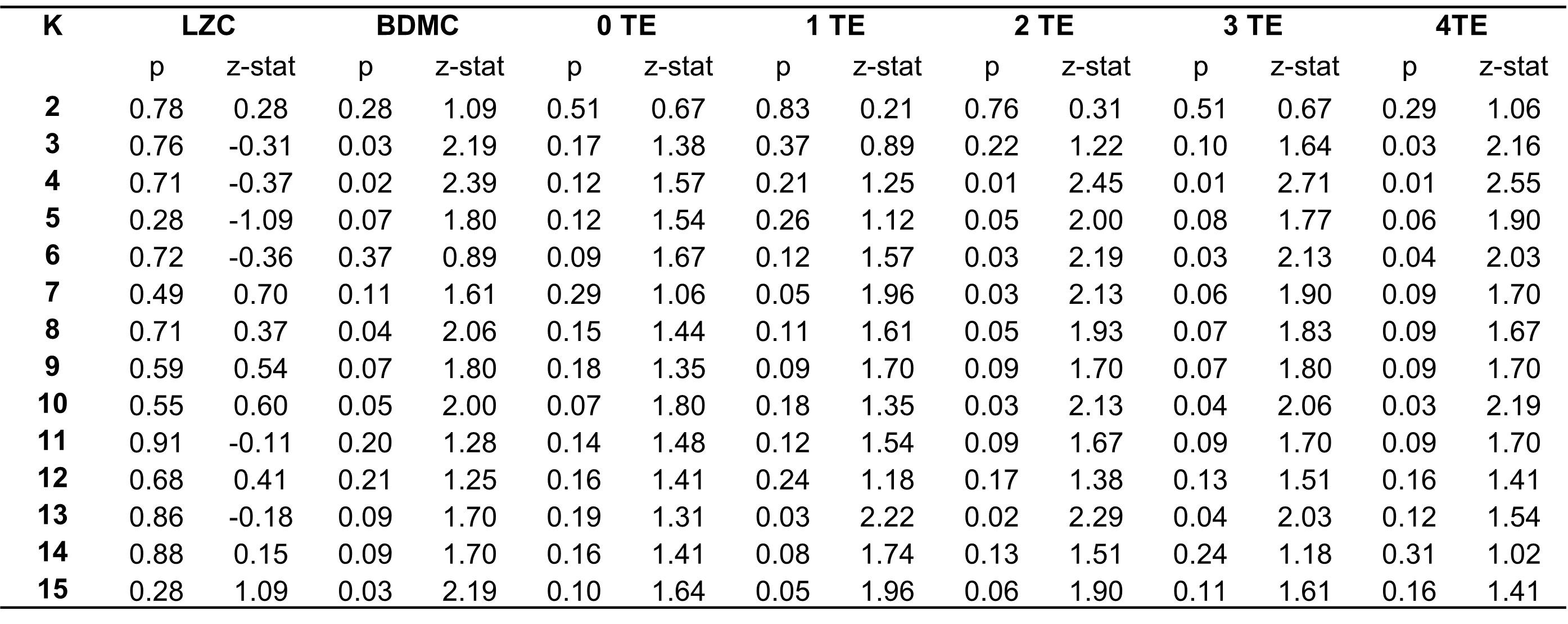
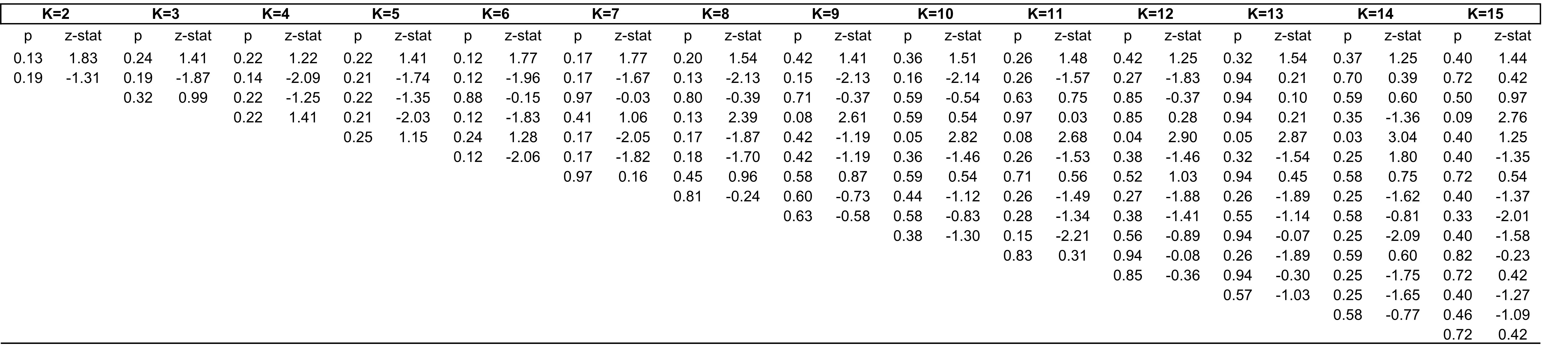
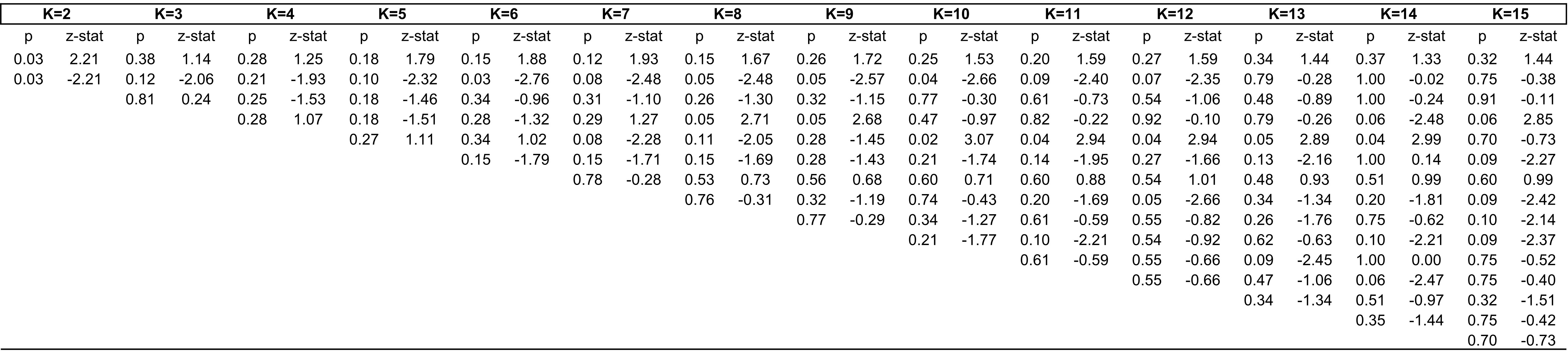
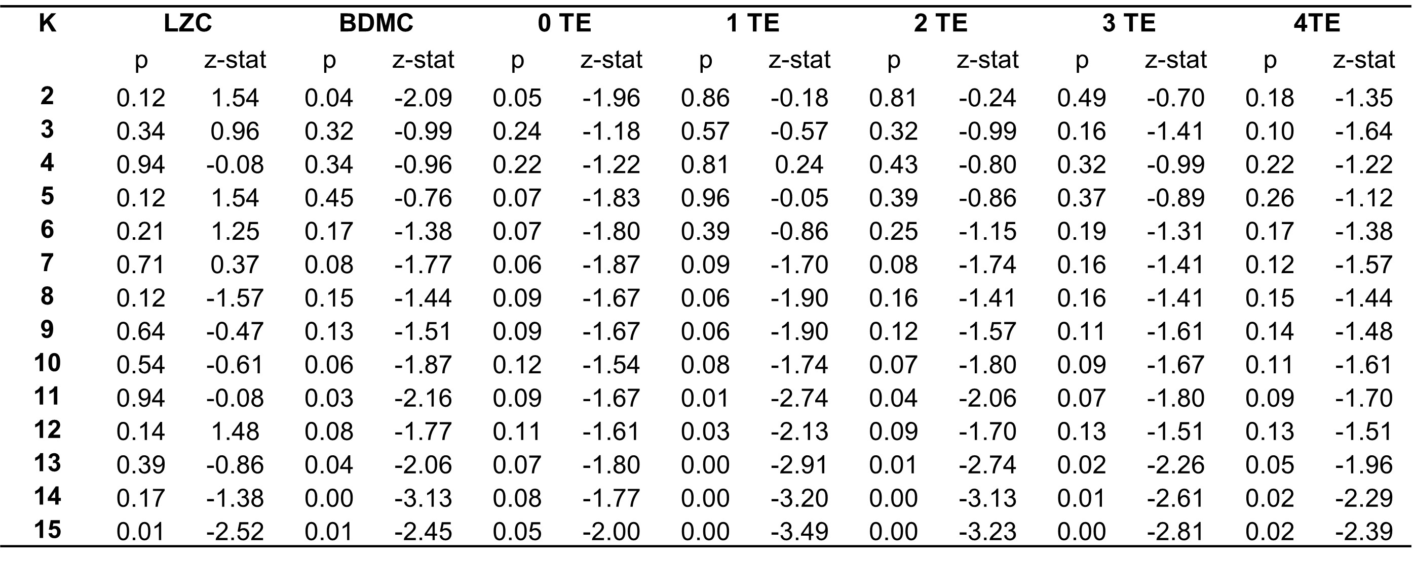
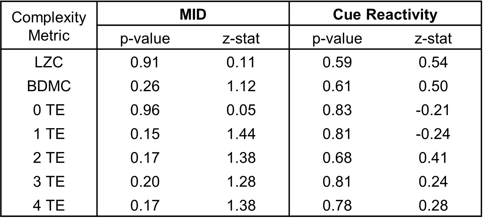
Metrics of brain state dynamics were computed for the entire task, but not the conditions of interest. The lifetime and probability of each state’s occurrence, and three information theoretic metrics – Lempel Ziv Complexity (LZC), Block Decomposition Method of Complexity (BDMC), and transition entropy – were computed as previously reported36 (Fig. 1). LZC and BDMC were computed on 4-bit binarized state timeseries via an LZC algorithm, LZ7637 and BDMC algorithms38–40, respectively.
Transition entropy for 0th – 4th order transitions was derived by first computing an Nth order (where N = 0–4) Markov Model representation of the sequence of brain states per person per condition, yielding a probability p for each type of transition present. The entropy (H) for each order of transition is then computed using Eq. 3:
$$H=-\sum (p.*{log}_{2}p)$$
3
Statistical analyses
All analyses were run in MATLAB2023a. Wilcoxon sign-rank tests evaluated the main effect of group on miFC- and dynamical FC-based metrics. P-values were FDR-corrected for multiple comparisons, and z-stats captured the direction of significant effects. Spearman’s correlations assessed relationships between z-stats (the test statistic for differences in miFC) and the pairwise sum of receptor availability, with p-values Bonferroni corrected for multiple comparisons.