Categorization scheme definition
In combination with expert radiologists, a categorization scheme is defined. That includes location, type of sequencing, type of weighting, and information about the use of different suppressions. The information contained in the categorization is helpful to get an overview of the content of the series and covers all preconditions necessary for the post-processing and feature extraction analyses.
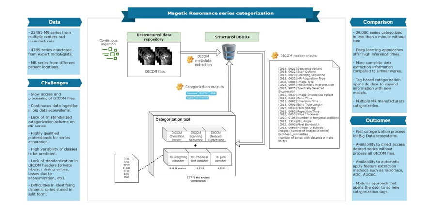
To comply with this scheme defined in Fig. 1, three different ML models have been developed (weighting classifier, chemical shift detector, and junk detector) together with a final algorithm that merges model outputs with raw values of DICOM headers.
This scheme is defined based on two main criteria. First, it is preferable to subtract information from a DICOM tag, that has 100% confidence, versus a model that includes a probabilistic approach. Secondly, ML models should have a single objective and must be as simple as possible. For instance, it is preferable to employ two separate models that individually classify weighting and junk than a unique model that classifies both weighting and junk simultaneously, where the number of target classes is duplicated.
The DICOM headers used in the schema of Fig. 1 to obtain the non-ML tags are “image orientation (patient)” (0020, 0037), “scanning sequence” (0018, 0020), “spectrally selected suppression” (0018, 9025) and “scan options” (0018, 0022).
It is relevant to note that one of the possible values that the “scanning sequence” DICOM tag can adopt, namely “research mode”, does not provide useful information for the MR series categorization. Therefore, these cases are treated as empty values in this DICOM tag, forcing the experts to manually label the scanning sequence field when this occurs.
In the “surnames” section of the schema, a combination of two different DICOM tags to detect the possible suppression in a series is applied. This is due to the different casuistry observed in the data around empty values of the two relevant tags (“Spectrally selected suppression”, in all cases, and “Scan Options”, when adopting the “FS” value). By combining them is it possible to identify the suppression in a larger set of cases.
Data
Data from the European H2020 PRIMAGE project was used for this paper [18]. The PRIMAGE project collects retrospective information from multiple clinical partners on Neuroblastoma and Diffuse Intrinsic Pontine Glioma (DIPG) in childhood. While DIPG images are specific to the brain, Neuroblastoma can appear in a wide variety of regions including abdominal, thoracic, and pelvic regions. The study images used were not only taken from different patient locations but also present a wide variety of MR manufacturers. The distribution of the manufacturers can be shown in Fig. 2.
In the PRIMAGE project, all DICOM metadata are extracted in the ingestion phase and stored in a semi-structured MongoDB database [19][20]. At the time of developing the categorization tool, 25,596 MR series are present in the platform, of which 4,666 series have been manually annotated by radiologists for model development and 1,286 for final system evaluation. The rest of the series is used to evaluate the final solution's performance on inference. Figure 3 shows the complete diagram of the MR series distribution.
Annotations
In order to annotate the MR series, the following filters have been used as an exclusion criterion before starting with the manual labeling by radiologists. On the one hand, the DICOM image type property (0008,0008), when adopting the "Derived" or "Secondary" values, was used to filter out post-processing pictures. On the other hand, the terms “ADC”, “preprocessed”, “registered” and “map” were filtered with a pattern-matching approach from the series description attribute (0008,103E). In both cases, these series were labeled as “Derived” (as shown in Fig. 3).
Table 1
Sample size by MR series category in dataset.
| Weighting | Number of manually labeled samples |
| T2W | 1326 |
| T1W | 1256 |
| DCE (Dynamic Contrast Enhance) | 496 |
| JUNK (localizer, calibration, others) | 484 |
| DWI (Diffusion weighted) | 480 |
| CHS (Chemical Shift) | 236 |
| STIR (Short Tau Inversion Recovery) | 236 |
| FLAIR (Fluid attenuated inversion recovery) | 113 |
| T2*W | 36 |
| PDW (Proton Density Weighted) | 2 |
| SW (Susceptibility weighted) | 1 |
Two experienced radiologists have performed semi-automatic labeling of the 4,666 DICOM MR series, supervising a traditional pattern-matching algorithm that classifies the weighting type. Table 1 displays the frequency of the manually labeled samples used to create the ML models.
The annotations are used to develop three different ML models (weighting classifier, chemical shift detector, and junk detector), but for their development not all the data in Table 1 is used as each particular model requires a specific set of annotations.
The MR series selected to develop a junk model capable of identifying useless data in the database includes the “JUNK” category as a positive class and the rest of the data are annotated as a negative class. The “JUNK” category not only has localizers and calibrations but also screenshots and images that are not useful for any desirable purpose (e.g., post-processing for the extraction of imaging biomarkers). The same occurs with the chemical shift model where the data corresponding to the “CHS” category is marked as a positive class and the rest as a negative class. The latter ML model will be used to enrich the categorization in the surname part of the scheme.
The MR series used for the development of the weighting model includes several of the manually annotated classified samples (T2W, T1W, DCE, DWI, STIR, FLAIR, T2*W). Categories "PDW" and "SW" presented an insufficient number of samples to train the models, so they had to be discarded from the weighting dataset. In addition, the "T2*W" category also showed an insufficient number of samples to train a robust model for this class. Therefore, it was decided to unify this category within the label "T2W" and to perform an a posteriori classification of the class in a declarative way by checking if the DICOM tag “scanning sequence” adopts the gradient echo (GR) value. If so, the label "T2W" was then replaced by "T2*W".
Models
3.4.1 Input features
The features used in the ML models developed in this study are a combination of those used in related works [15], [16] and others proposed by experienced radiologists. Only features automatically generated by machines are included, which have a high percentage of occurrence in the data used (with less than 15% of missing values in the global of all the series). In addition to the DICOM metadata indicated above, two additional features have also been included as a result of a feature engineering process. They correspond to the number of images in a series (“Images”) and to the number of series with Euclidean distance equal to 0 in the same MR study (“Euclidean_similarities”). The list of input features is shown in Table 2.
Table 2
Input features for ML model development.
| Categorical Features | Numerical Features |
| (0018, 0021) Sequence Variant | (0018, 0081) Echo Time |
| (0018, 0022) Scan Options | (0018, 0082) Inversion Time |
| (0018, 0020) Scanning Sequence | (0018, 0091) Echo Train Length |
| (0018, 0023) MR Acquisition Type | (0028, 0030) Pixel Spacing |
| (0008, 0008) Image Type | (0018, 0080) Repetition Time |
| (0028, 0004) Photometric interpretation | (0018, 0050) Slice Thickness |
| (0018, 9025) Spectrally Selected Suppression | (0020, 0105) Number of temporal positions |
| (0020, 0037) Image Orientation Patient | (0018, 1314) Flip Angle |
| | (0018, 0095) Pixel Bandwidth |
| | (0018, 0086) Number of Echoes, (Optionally studied (0019, 10A9)) |
| | Images (number of images in a series) |
| | Euclidean_similarities (number of series with Euclidean distance equal to 0 in the same study) |
A dynamic MR series constitutes the union of different individual series in one with a specific objective. For example, the DCE series is a combination of multiple T1W series across time with the purpose of observing the effect of contrast as a function of time. For a model, it is easy to detect a dynamic series based on the number of images contained if they are stored in the combined form but, as shown in Fig. 4, in the divided or split way it is very difficult to detect if a T1W series belongs to a DCE combination or if it is a unique T1W acquisition.
The “Euclidean_similarities” feature can detect composite series that are stored in a split way within the same study. Composite series usually keep the same acquisition parameters as their internal series except one or two of them, such as contrast or time. For this reason, a selection of variables has been made to calculate the Euclidean distance among the different series. This method provides the number of identical series within the same study. The characteristics used for the calculation of this Euclidean distance are “Scanning Sequence”, “Orientation Patient”, "Echo Time", "Flip Angle", "Repetition Time", "Pixel Bandwidth", "Number of Images", "Number of temporal positions" and "Slice Thickness".
Other DICOM tags have been studied and discarded due to complex problems in the system but may be desirable in future work. One tag to consider is the diffusion b-value (0018, 9087) of the first and last image in the series. This information could be very helpful to alternatively classify the DWI series.
3.4.2 Transformations
As commonly done when training ML algorithms, several feature transformations have been applied to maximize the learning in trained models. The transformations per feature can be seen in Table 3.
Table 3
Transformations of input features. Abbreviations and definitions: SK (segmented k-space), SS (steady state), SP (spoiled), OSP (oversampling phase), PER (phase encode reordering), RG (respiratory gating), CG (cardiac gating), PPG (peripheral pulse gating), FC (flow compensation), PFF (partial Fourier - frequency), PFP (partial Fourier - phase), SP (spatial presaturation), FS (fat suppression), SE (spin echo), GR (gradient echo), IR (inversion recovery), EP (echo planar), RM (research mode), RGB (red, green, blue), FAT (fat suppression).
| DICOM Features | Preprocessing |
| (0018, 0021) Sequence Variant | One hot encoding for values SK, SS, SP, OSP. |
| (0018, 0022) Scan Options | One hot encoding for values PER, RG, CG, PPG, FC, PFF, PFP, SP, FS. |
| (0018, 0020) Scanning Sequence | One hot encoding for values SE, GR, IR, EP, RM. |
| (0018, 0023) MR Acquisition Type | Categorical label encoded. |
| (0008, 0008) Image Type | One hot encoding for values DERIVED, SECONDARY, LOCALIZER, ADC, SCREENSAVE. |
| (0028, 0004) Photometric interpretation | Binary value depending if contains RGB. |
| (0018, 9025) Spectrally Selected Suppression | Binary value depending if contains FAT. |
| (0020, 0037) Image Orientation Patient | Transformation from numeric vectors to categories Sagittal, Axial, Coronal. One hot encoded transformation. |
| (0018, 0081) Echo Time | Round the two numeric values to the first decimal. Label encoded transformation. |
| (0018, 0082) Inversion Time | Set empty values simulating infinity with 100000000 value. |
| (0018, 0091) Echo Train Length | - |
| (0028, 0030) Pixel Spacing | Categorical label encoded. |
| (0018, 0080) Repetition Time | - |
| (0018, 0050) Slice Thickness | - |
| Number of images in series (custom feature) | - |
| (0018, 1314) Flip Angle | Set empty values simulating infinity with 100000000 value. |
| (0018, 0095) Pixel Bandwidth | Set empty values simulating infinity with 100000000 value. |
| (0018, 0086) Number of Echoes | Set empty values simulating infinity with 100000000 value. |
| (0020, 0105) Number of temporal positions | Set empty values simulating infinity with 100000000 value. |
Different transformations are applied on the target variable depending on the model developed. In the case of the weighting model, the different categories are transformed with a label encoder. For the junk classifier, a binary encoding is applied (where a value of “1” corresponds to the “JUNK” category and the rest of the categories adopt a value of ”0”). The same strategy is followed in the chemical shift model.
3.4.4 Feature selection
A total of 43 transformed features have been generated after the application of feature engineering with all the transformations listed in Section 3.4.2 Transformations. To select the most relevant features and reduce as much as possible the number of inputs to be used in the models, the Boruta feature selection algorithm [21] has been applied. As it is a supervised algorithm, it has been applied to each model independently (weighting, junk, and chemical shift).
The Boruta algorithm has been chosen over other alternatives because it is a feature detection algorithm that does not require input parameters and thus avoids the user having to make decisions regarding the cut-off threshold for separating the features to keep from the ones to remove. Boruta's only requirement for its application is the choice of the ML algorithm to be used internally for selection. Typically, a RandomForest is used, due to its robustness to data with anomalies or noise, and its ability to detect non-linear relationships between features [22]. In addition, and before applying the Boruta algorithm together with the RandomForest for selection, an imputation of the missing values that may exist with the K-Neighbours algorithm has been performed, since a RandomForest does not allow the presence of missing values for its execution.
Boruta outputs a classification into three groups of features according to the level of certainty in keeping the variables in a predictor. Only the features of the group with certainty to be eliminated have been filtered out, thus keeping the features recommended to be kept and the features of which there is no certainty to be kept or eliminated. This has resulted in a total of 26 features selected for each model.
3.4.5 Algorithms
An intrinsic characteristic of the metadata contained in the DICOM headers is the absence of some particular tags and labels due to the great heterogeneity of the standard, especially if the series come from different hospitals and machines. It is common to encounter missing DICOM tags when working in environments with heterogeneous sources.
The most common classification algorithms cannot deal with data with missing or empty tags and/or values. For this reason, they are often combined with value imputation algorithms capable of detecting patterns. The addition of an imputation model means an increase in the complexity of the overall system and an increase in inference latencies per sample. In big data environments, inference times could be critical and even more so when dealing with medical images, which are costly data to process. For this reason, it has been proposed to use the Catboost algorithm [23], as its ability to deal with missing data, its fast inference times with both CPU and GPU, and its good performance in non-linear detection problems, make it a perfect fit with the desired requirements.
This decision was made after iteratively optimizing the results of a RandomForest with a KNN imputer and a Catboost classifier [24]. The low variability in the scores and the high performance in the obtained results were the main reasons in choosing this feature selection and model combination in this study, resulting in a simple, stable, robust and explainable tool.