Continental subduction below oceanic plates and associated emplacement of far-travelled ophiolite sheets remain enigmatic chapters in global plate tectonics. Numerous ophiolite belts on Earth exhibit continental rocks that experienced subduction-related high pressure-low temperature (HP-LT) metamorphism and subsequent exhumation coeval with the emplacement of ophiolites. However, the link between continental subduction dynamics and ophiolite emplacement is poorly understood. Here we combine data collected from ophiolite belts worldwide with thermo-mechanical simulations of continental subduction dynamics to show the causal link between the exhumation of subducted continental crust and ophiolite emplacement. Our results reveal that buoyancy-driven extrusion of subducted crust triggers necking and breaking of the overriding oceanic upper plate. This process is fundamental for the formation of a far-travelled ophiolite sheet that is separated from the oceanic domain by the exhumed, HP-LT continental upper crust. Our results indicate that the exhumation of the subducted continental crust and far-travelled ophiolite sheet emplacement are inseparable processes and thus shed light on one of the most mysterious aspect of plate tectonics.
Article
Extrusion of subducted crust explains the emplacement of far-travelled ophiolites
https://doi.org/10.21203/rs.3.rs-44696/v1
This work is licensed under a CC BY 4.0 License
Journal Publication
published 08 Mar, 2021
Version 1
posted
You are reading this latest preprint version
continental subduction
ophiolite emplacement
thermo-mechanical simulations
buoyancy-driven extrusion
plate tectonics
The search for finding physical mechanisms that explain how dense oceanic lithosphere, referred to as ophiolite, is emplaced (obducted) on top of lighter continental plates has prompted a long-standing scientific discussion1–3. Ophiolites may be accreted to continents by being scraped off from the subducting oceanic lower plate 1,4, or emplaced on top of the continent in a continental lower plate - oceanic upper plate subduction setting 5,6. In the latter case, ophiolite belts exhibit HP-LT metamorphic units structurally underlying the ophiolite sheet (Fig. 1a, b, c). These HP-LT units predominantly consist of continental upper crust that represents the former passive margin of the subducting continent 7–9. The subduction and exhumation of these units appear to be a relatively short-lived process, as evidenced by the characteristic duration of 10–30 Myr for the subduction-exhumation cycle recorded by the metamorphic rocks (Fig. 1e). The exhumed continental units are typically found in between the obducted ophiolite sheet and the rest of the oceanic domain (open ocean or suture zone of the former ocean), thus separating a far-travelled ophiolite sheet from its root (Fig. 1a, b). Far-travelled ophiolite sheets are up to 10 km thick, and their average width is 50–55 km (Fig. 1e), suggesting that their dimensions are mechanically limited during emplacement.
Models of ophiolite emplacement hence have to account for 1) short-lived continental subduction below the oceanic upper plate followed by exhumation of the subducted upper crust, and 2) matching the observed dimensions of ophiolite sheets. Recent numerical modelling studies achieved these conditions by imposing convergence to reach the state of continental subduction, and subsequently imposing divergence to exhume the continental margin and thin the oceanic upper plate 6,12. These models however do not lead to nappe formation in the subducted continental crust, which is a key feature of natural systems and is commencing once the oceanic plate is thrust on top of the continent 7,10,13. As such, upper crustal decoupling and nappe formation seems to be critical for inducing uplift on top of the rising thrust sheet(s) which in turn may lead to gravity-driven extension in the oceanic upper plate, thus facilitating simultaneous ophiolite emplacement and crustal exhumation 14–16.
Here we combine numerical thermo-mechanical simulations of oceanic upper plate-continental lower plate subduction systems and data acquired in ophiolite belts worldwide to unravel the physical processes that explain the structure of ophiolite belts. We highlight the genetic link between the exhumation of the subducted continental crust and the emplacement of far-travelled ophiolite sheets, and further identify the key parameters controlling this process.
Modelling strategy
We designed 2D thermo-mechanical numerical simulations governed by momentum, mass, and heat conservation equations and a visco-elasto-plastic rheological model (see Methods for details of numerical modeling techniques and further model setup description). A total plate convergence velocity of 3 cm/yr is achieved by prescribing constant normal inflow velocities of |Vin|=1.5 cm/yr along the upper 140 km of the two model sides. Mass conservation is satisfied by gradually increasing outflow below 140 km (Fig. 2a). The top boundary of the model is a true free surface 17. The model geometry is inspired by reconstructions of pre-obduction geodynamic settings where intra-oceanic subduction is initiated relatively close (< 400 km) to the continental passive margin, which arrives to the subduction zone after ~ 10 Myr of oceanic subduction 18–20. Subduction is designed to initiate along an inclined weak zone (equivalent of an oceanic detachment) close to the mid-ocean ridge to achieve a right-dipping subduction zone and a thermally young ophiolite front, in agreement with natural ophiolite belts 21. A simplified continental passive margin geometry is implemented by linearly decreasing crustal thickness over the distance of 200 km (Fig. 2a). The continental basement is divided in two parts (upper and lower crust) constituted by different materials (Fig. 2a and Table 1), which introduces a decoupling level at the base of the upper crust (Fig. 2a). A resolution test was performed to verify the robustness of the model results (Supplementary Fig. 1).
General evolution of the reference model
Intra-oceanic subduction initiation is followed by the subduction of oceanic lithosphere until 10 Myr. The passive margin of the continent then starts to subduct below the oceanic upper plate (i.e. obduction) (Fig. 2b), and experiences HP-LT metamorphism up to eclogite facies conditions (Fig. 2c). The 3 km thick sedimentary cover of the passive margin partially subducts with the rest of the continental lithosphere, but is largely stacked and accreted to the front of the oceanic upper plate (Fig. 2). After reaching eclogite facies conditions, the burial velocity of the upper crust decreases from ~ 3 cm/yr at 18 Myr to near zero at 23 Myr. Consequently, the upper crust starts to decouple from the lower crust and the lithospheric mantle. Decoupling results in the localization of a major reverse-sense shear zone along which the subducted upper crust is extruded upwards and leftwards (Figs. 2d). The oceanic upper plate undergoes gravity-driven extension when being pushed up by the extruding thrust sheet. Extension leads to the breaking of the oceanic upper plate, which enables the continental upper crust to be rapidly extruded to the surface, separating a 50 km wide and maximum 13 km thick far-travelled ophiolite sheet from the rest of the oceanic lithosphere (Figs. 2d, e).
Ductile nappe formation: the onset of exhumation
Burial of continental crust below a denser oceanic plate leads to a progressive increase of the buoyancy force that resists subduction despite the continuously imposed plate convergence. From ~ 21 Myr (i.e. after 11 Myr of continental subduction) the velocity of the subducting continental upper crust becomes near zero, while the lower crust and the lithospheric mantle still subducts at ~ 1.5 cm/yr (Fig. 3a). This kinematic setting leads to an increase of deviatoric stress within the lower crust, which meets the conditions for strain localization by thermal softening 22. As a result, a major reverse-sense shear zone develops and exhibits strain rates of > 10− 13 s− 1 (Fig. 3a). The shear zone is initially low-angle, and propagates along the base of the upper crust, which is the weakest horizon in the continental crust (Figs. 2a, 3a). The shear zone thus facilitates decoupling between the crustal layers, which is further accommodated by distributed deformation (folding) at a strain rate of ~ 10− 14 s− 1 in the entire subducted upper crust.
Interplay between crustal extrusion and upper plate necking
Upper crustal decoupling and nappe formation results in uplift, which triggers extension of the oceanic upper plate over a 50 km wide zone (Fig. 3a). Initial extension of the upper plate leads to the formation of normal faults and to the normal-sense reactivation of the original plate boundary thrust (Fig. 3a).
Further strain localization leads to the connection of the two flat reverse-sense shear zone segments by a steeper ramp segment. This structure separates very-low-grade to non-metamorphic upper crust from the low-grade to eclogite facies upper crust (Fig. 3b). The accelerating extrusion of the upper crust (from 0.5-1 cm/yr until 24.5 Myr to 1.5-3 cm/yr from 25 Myr) is accommodated by increasing displacement along the right-and left-dipping extensional shear zones and leads to the necking of the oceanic upper plate (Figs. 3b, c). Through this process a sheet of oceanic lithosphere (the future far-travelled ophiolite) gets disconnected from the oceanic plate along the left-dipping normal fault, which joins the roof segment of the main thrust in depth (Fig. 3b). Subsequently, the far-travelled ophiolite sheet is emplaced on top of the continent and transported to the left via the roof thrust as dictated by further crustal extrusion (Fig. 3c).
Key parameters controlling crustal extrusion and far-travelled ophiolite emplacement
Extensive tests have been performed from the reference model to determine key parameters that control the extrusion of the upper crustal thrust sheet, which is instrumental for the necking of the upper plate and the emplacement of far-travelled ophiolite sheets (Fig. 4). In particular, we evaluated the impact of shear heating and variations of crustal rheology of the subducting plate on the process of nappe formation.
The model without shear heating (Fig. 4) shows, that strain localization and nappe formation fails to initiate, or is significantly delayed compared to the reference model (Fig. 3). In this case the coupling between the upper crust and the subducting lithosphere is too high to allow for nappe formation and its subsequent extrusion. Instead, buoyancy force leads to the underplating of the subducted upper crust. This demonstrates that shear heating is essential for strain localization and nappe formation.
In the reference model, a decoupled crustal rheology is achieved by using Westerly granite flow law 24 for the continental upper crust, and mafic granulite flow law 25 for the lower crust (Fig. 2a). Using a stronger Maryland diabase flow law 23 for the upper crust results in a more coupled, stronger crustal rheology (Fig. 2a). This prevents upper crustal decoupling after reaching eclogite facies conditions, and inhibits subsequent nappe formation and extrusion (Fig. 4b). Instead, slightly deeper upper crustal subduction and enhanced underplating occurs compared to the reference model.
A more coupled, but relatively weak crustal rheology can be achieved by decreasing the strength of the continental lower crust (Figs. 2a, 4c). Such rheology results in the decoupling of the entire continental crust from the lithospheric mantle rather than the decoupling of the upper crust from the lower curst (Fig. 4c). This leads to distributed folding and thrusting in the lower plate rather than localized nappe formation and extrusion of the subducted upper crust. Our results thus indicate that both strong (Fig. 4b) and weak (Fig. 4c) coupled crustal rheologies inhibit upper crustal extrusion and associated far-travelled ophiolite emplacement. We further tested different types of decoupled crustal rheological models to determine the effect of smaller compositional or thermal differences. Results show that slight variations in the thermal and material properties lead to different timing and thus position of crustal decoupling, which is reflected in different amounts of underplated continental upper crust below the oceanic upper plate (Supplementary Fig. 2). Rheology and coupling of the continental crust is hence a key factor that controls nappe formation, upper crust extrusion, and eventual upper plate necking.
Comparison to natural ophiolite belts
Our reference model displays many first-order features of natural ophiolite belts that are related to continental subduction below an oceanic upper plate. It produces a far-travelled ophiolite sheet as the structurally highest unit, separated from its root by subducted and then exhumed HP-LT continental rocks, and underlain by accreted low-grade to non-metamorphic sedimentary cover units (Figs. 1a, b, 3c). The prograde P-T ratio and peak P-T conditions recorded by the subducted upper crust in our model (4 MPa/°C and ~ 2 GPa at 500–600 °C, respectively) are average values compared to those of natural cases (Figs. 1c, 2d, Supplementary Table 1). The duration of the model subduction-exhumation cycle (15–20 Myr) is in agreement with the well-constrained ophiolite belts like Oman or New Caledonia, and appears to be slightly shorter than the sites where subduction and/or exhumation of the continental formations is poorly dated or debated (e.g. Brooks Range, Hellenides-Dinarides, Southern Ural) (Fig. 1e, Supplementary Note 1, Supplementary Table 2). Observations such as post-subduction ductile to brittle extensional deformation 10,26, or the coexistence of opposite shear sense directions in the former passive margin units 9,27 fit well to the structural evolution of our model that involves top-left shearing (thrusting) during burial and both top-left and top-right shearing during exhumation (normal faulting) (Fig. 3). The width of the far-travelled ophiolite sheet (50 km) predicted by the reference model agrees very well with the average width (53 km) of natural ophiolite belts (Fig. 1e, Supplementary Note 1). The geometry and time evolution of our model also allows comparison with the currently active continental subduction of the Australian continental margin below the oceanic Banda arc. The Australian continental margin have been subducting for ~ 10 Myr 28, which roughly equals the duration of upper crustal subduction in our reference model. Reconstruction of the stacked sedimentary cover showed that 215–230 km of continental lithosphere is subducted, and only the uppermost 2 km of sedimentary cover was accreted to the upper plate 29. Hence the present-day structure and dimensions of the Australian continental subduction are very similar to those of our reference model at 20–23 Myr snapshots (Fig. 2c).
Our results have important implications for the dynamics of ophiolite emplacement in oceanic upper plate-continental lower plate subduction systems, and thus may be widely applied to explain geological observations in natural ophiolite belts. While plate kinematic changes may play an important role in initiating intra-oceanic subduction 30, or in the cessation of contraction at continental subduction zones 6, we show that the emplacement of far-travelled ophiolite sheets can result from syn-convergence, buoyancy-driven decoupling and upward extrusion of the subducted continental upper crust accommodated by the necking of the oceanic upper plate. Extrusion of the subducted upper crust requires nappe formation. In agreement with previous studies 22,31, results show that shear heating is an important mechanism that facilitates strain localization and nappe formation. The precise reproduction of smaller scale nappes (nappe thickness of several kilometers) which is often observed in case of continental subduction 7,10 would require very high-resolution numerical modeling and built-in heterogeneities inside the upper crust to localize shear zones at multiple horizons 32,33. Our results also support that crustal decoupling and exhumation may take place with different timing and position in the subducted continent depending on the rheology of the continental crust 34,35. Variations in thermal or compositional properties thus might control the surface preservation (exhumation) or the subduction and recycling of different types of continental passive margins 36–38.
Numerous natural ophiolites show evidences for supra-subduction zone magmatism in the upper plate following intra-oceanic subduction initiation, which results in thermally younger, thus thinner upper plates 39–42. Our model does not account for such effects and hence may overestimate upper plate thickness. Thinner upper plates may result in flatter continental subduction that may lead to crustal decoupling and upper plate necking further away from the ophiolite front. If so, the size of the resulting far-travelled ophiolite sheets would be comparable to the widest far-travelled ophiolite sheets in Oman and Anatolia (80–150 km).
The currently subducting Australian plate below the oceanic Banda arc provides an exciting example for a prospective future ophiolite belt. As more than 200 km of continental crust has already subducted below the oceanic plate 29, it most likely reached eclogite facies conditions. Based on our model, decoupling of the Australian upper crust has already initiated, or will initiate in the geological near future. If decoupling is followed by nappe formation, the extrusion of the upper crust and simultaneous necking of the oceanic upper plate may lead to far-travelled ophiolite emplacement.
Numerical modelling
The presented thermo-mechanical models were obtained by solving the conservation equation for a steady state momentum, transient heat conservation and incompressible mass conservation equations:
![]()
![]()
![]()
where v is the velocity vector, T is the temperature, k is the thermal conductivity, ρ is the density, cp is the heat capacity, Qr is the radiogenic heat production, τ is the deviatoric stress tensor, ![]() is the deviatoric strain rate tensor, P is the pressure and g is the gravity acceleration vector. The term
is the deviatoric strain rate tensor, P is the pressure and g is the gravity acceleration vector. The term ![]() describes the production of heat by visco-plastic dissipation (shear heating).
describes the production of heat by visco-plastic dissipation (shear heating).
The density field evolves according the following equation of state:
![]()
whereρ0 is the reference density, α is the thermal expansivity, β is the compressibility, T0 and P0 are the reference temperature and pressure which were respectively set to 0 C and 105 Pa.
The effective viscosity (![]() ) relates the deviator stress and strain rate tensor in the following fashion:
) relates the deviator stress and strain rate tensor in the following fashion:
![]()
and is computed in order to satisfy a visco-elasto-plastic rheological model:
![]()
where the v, e, and p superscripts correspond to viscous, elastic and plastic portions and the surperscripts dis and Peierls refers to the dislocation and Peierls creep mechanisms.
The viscous strain rate is computed as:
![]()
where A is a pre-factor, Q is the activation energy, n is the stress exponent R is the universal gas constant and f is a correction factor 43. The subscripts II stand for the square root of the second tensor invariant. For rheological parameters used in the reference model, see Table 1. The elastic strain rate is written as:
![]()
where G is the shear modulus (set to 1010 Pa).
The plastic strain rate takes the form of:
![]()
where ![]() is the friction angle and
is the friction angle and ![]() is the cohesion (for friction angle and cohesion values of the reference model see Table 1). We do not apply any plastic strain softening.
is the cohesion (for friction angle and cohesion values of the reference model see Table 1). We do not apply any plastic strain softening.
In the mantle lithosphere, the Peierls mechanism is also activated and its strain rate is computed as:
![]()
where the effective strain rate is spelled as:
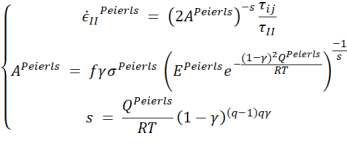
where the parameters s is the effective stress exponent (T-dependent), QPeierls is the activation energy (=540 J/mol), σPeierls is the Peierls stress (=8.5.109 Pa), EPeierls (=5.7.1011 s-1), q (=2.0), andγ (=0.1) 44. Peierls creep stress is computed using a regularised formulation 45.
The temperature is kept constant at both the upper (0oC) and lower boundaries (1330oC) and the heat flow is set to 0oC across the right and left boundaries. A plate convergence rate of 3 cm/year is achieved by prescribing constant normal inflow velocities of |Vin|=1.5 cm/year along the upper 140 km of the two model sides, while mass conservation is satisfied by gradually increasing outflow below 140 km. The shear stress is set to zero along the left, right and lower boundaries. The upper boundary is a true free surface that dynamically evolves with time 17.
The initial temperature field is obtained by solving the steady state heat equation (neglecting shear heating) using reference thermal parameters (Table 1), excepted below the lithospheric mantle where the conductivity was set artificially high in order to produce a quasi-adiabatic asthenosphere. The initial topography is set to 0 km.
The conservation equations are discretized using a finite difference/marker-in-cell technique 46. The global linearized systems of equations are solved using a direct-iterative method 47. Non-linear iterations are used at both local and global levels. At the local level, Newton iterations ensure exact partitioning of strain rates and correct evaluation of effective viscosity 48,49. At the global level, Picard iterations are employed to best-satisfy mechanical equilibrium equations (to an absolute tolerance of 10-6 and within a maximum of 20 iterations).
|
ρ (kg.m− 3) |
k (W.m− 1.K− 1) |
Qr (W.m− 3) |
α (K− 1) |
C (MPa) |
ϕ |
A (Pa-n.s− 1) |
n |
Q (J.mol− 1) |
|
|---|---|---|---|---|---|---|---|---|---|
|
Sedimentary cover (mica) |
2700 |
2.55 |
2.9e-6 |
3.0e-5 |
10 |
15 |
1.0e-138 |
18 |
51.0e3 |
|
Continental upper crust (Westerly granite) |
2750 |
2.8 |
1.65e-6 |
3.0e-4 |
10 |
30 |
3.1623e-26 |
3.3 |
186.5e3 |
|
Continental lower crust (mafic granulite) |
2900 |
2.8 |
1.65e-6 |
3.0e-4 |
10 |
30 |
8.8334e-22 |
4.2 |
445.0e3 |
|
Oceanic crust (Maryland diabase) |
2900 |
3.0 |
1.0e-10 |
3.0e-5 |
10 |
30 |
3.2e-20 |
3.0 |
276.0e3 |
|
Lithospheric mantle (dry olivine) |
3300 |
3.0 |
1.0e-10 |
3.0e-5 |
10 |
30 |
1.1e-16 |
3.5 |
530.0e3 |
|
Asthenosphere (dry olivine) |
3300 |
3.0 |
1.0e-10 |
3.0e-5 |
10 |
30 |
1.1e-16 |
3.5 |
530.0e3 |
|
Weak zone (serpentinite) |
2900 |
3.0 |
1.0e-10 |
3.0e-5 |
0 |
30 |
4.4738e-38 |
3.8 |
8.9e3 |
Model geometry
The computational domain is a cross section of 1330 × 410 km. The model resolution is 1 km in both directions. The initial compositional geometry is inspired by reconstructions of pre-obduction geodynamic settings. It contains an oceanic domain (660 km wide) with a spreading ridge and a tilted weak zone in the center that ensures left-dipping intra-oceanic subduction initiation. The thermal structure of the oceanic lithosphere is calculated by applying a half-space cooling age model from 1.5 Myr at the center to 50 Myr at the edges of the ocean. The oceanic crust is 6 km thick and is overlain by a layer of uppermost sedimentary cover that linearly thickens from the ridge (0 km) towards the right edge of the continental domain (3 km). The transition from the continent to the ocean is defined by a passive margin geometry where the continental upper and lower crust linearly thin from 30 km to 5 km over the distance of 200 km. The uppermost sedimentary cover layer has a constant 3 km thickness over the continental domain.
Data availability
Model output files that support the results of this study are stored in the data repository of Utrecht University and are available upon request.
Data availability
Model output files that support the results of this study are stored in the data repository of Utrecht University and are available upon request.
Acknowledgments
The research leading to these results has received funding from the European Union's MSCA-ITN-ETN Project SUBITOP 674899. Numerical simulations were performed on the Utrecht University cluster Eejit. Thanks are due to Jeroen van Hunen and Cedric Thieulot for discussions that helped to initiate the project.
Author contributions
K.P. conceived the research idea. T.D. and P.Y. designed the thermo-mechanical numerical code. A.A, P.Y., T.D., and K.P. designed the model setup. K.P. conducted the numerical simulations and interpreted the results together with P.Y., T.D., and E.W. All authors discussed the results and interpretations, and contributed to writing the paper.
Competing interests
The authors declare no competing interests.
- Coleman, R. Plate tectonic emplacement of upper mantle peridotites along continental edges. Journal of Geophysical Research 76, 1212–1222 (1971).
- Dewey, J. Ophiolite obduction. Tectonophysics 31, 93–120 (1976).
- Agard, P. et al. Obduction: Why, how and where. Clues from analog models. Earth and Planetary Science Letters 393, 132–145 (2014).
- Oxburgh, E. Flake tectonics and continental collision. Nature 239, 202–204 (1972).
- Boudier, F., Ceuleneer, G. & Nicolas, A. Shear zones, thrusts and related magmatism in the Oman ophiolite: initiation of thrusting on an oceanic ridge. Tectonophysics 151, 275–296 (1988).
- Duretz, T. et al. Thermo-mechanical modeling of the obduction process based on the Oman ophiolite case. Gondwana Research 32, 1–10 (2016).
- Kilias, A. et al. Alpine architecture and kinematics of deformation of the northern Pelagonian nappe pile in the Hellenides. (2010).
- Yamato, P. et al. New, high-precision P–T estimates for Oman blueschists: implications for obduction, nappe stacking and exhumation processes. Journal of Metamorphic Geology 25, 657–682 (2007).
- van Hinsbergen, D. J. et al. Tectonic evolution and paleogeography of the Kırşehir Block and the Central Anatolian Ophiolites, Turkey. Tectonics 35, 983–1014 (2016).
- Searle, M. P. Structural geometry, style and timing of deformation in the Hawasina Window, Al Jabal al Akhdar and Saih Hatat culminations, Oman Mountains. GeoArabia 12, 99–130 (2007).
- Patriat, M. et al. New Caledonia obducted Peridotite Nappe: offshore extent and implications for obduction and postobduction processes. Tectonics 37, 1077–1096 (2018).
- Hässig, M., Rolland, Y., Duretz, T. & Sosson, M. Obduction triggered by regional heating during plate reorganization. Terra Nova 28, 76–82 (2016).
- Pourteau, A. et al. Neotethys closure history of Anatolia: insights from 40Ar–39Ar geochronology and P–T estimation in high-pressure metasedimentary rocks. Journal of Metamorphic Geology 31, 585–606 (2013).
- Lagabrielle, Y., Chauvet, A., Ulrich, M. & Guillot, S. Passive obduction and gravity-driven emplacement of large ophiolitic sheets: The New Caledonia ophiolite (SW Pacific) as a case study? Bulletin de la Société géologique de France 184, 545–556 (2013).
- Agard, P., Searle, M. P., Alsop, G. I. & Dubacq, B. Crustal stacking and expulsion tectonics during continental subduction: P-T deformation constraints from Oman. Tectonics 29 (2010).
- Chemenda, A. I., Mattauer, M. & Bokun, A. N. Continental subduction and a mechanism for exhumation of high-pressure metamorphic rocks: new modelling and field data from Oman. Earth and Planetary Science Letters 143, 173–182 (1996).
- Duretz, T., May, D. A. & Yamato, P. A free surface capturing discretization for the staggered grid finite difference scheme. Geophysical Journal International 204, 1518–1530 (2016).
- Searle, M. & Cox, J. Tectonic setting, origin, and obduction of the Oman ophiolite. Geological Society of America Bulletin 111, 104–122 (1999).
- Maffione, M. & van Hinsbergen, D. J. Reconstructing plate boundaries in the Jurassic neo-Tethys from the east and west Vardar ophiolites (Greece and Serbia). Tectonics 37, 858–887 (2018).
- Maffione, M., van Hinsbergen, D. J., de Gelder, G. I., van der Goes, F. C. & Morris, A. Kinematics of Late Cretaceous subduction initiation in the Neo-Tethys Ocean reconstructed from ophiolites of Turkey, Cyprus, and Syria. Journal of Geophysical Research: Solid Earth 122, 3953–3976 (2017).
- Maffione, M. et al. Dynamics of intraoceanic subduction initiation: 1. Oceanic detachment fault inversion and the formation of supra-subduction zone ophiolites. Geochemistry, Geophysics, Geosystems 16, 1753–1770 (2015).
- Kiss, D., Podladchikov, Y., Duretz, T. & Schmalholz, S. M. Spontaneous generation of ductile shear zones by thermal softening: Localization criterion, 1D to 3D modelling and application to the lithosphere. Earth and Planetary Science Letters 519, 284–296 (2019).
- Carter, N. L. & Tsenn, M. C. Flow properties of continental lithosphere. Tectonophysics 136, 27–63 (1987).
- Hansen, F. & Carter, N. in The 24th US Symposium on Rock Mechanics (USRMS). (American Rock Mechanics Association).
- Ranalli, G. Rheology of the Earth. (Springer Science & Business Media, 1995).
- Rawling, T. J. & Lister, G. S. Large-scale structure of the eclogite–blueschist belt of New Caledonia. Journal of Structural Geology 24, 1239–1258 (2002).
- Porkoláb, K. et al. Cretaceous-Paleogene tectonics of the Pelagonian zone: inferences from Skopelos island (Greece). Tectonics (2019).
- Keep, M. & Haig, D. W. Deformation and exhumation in Timor: Distinct stages of a young orogeny. Tectonophysics 483, 93–111 (2010).
- Tate, G. W. et al. Australia going down under: Quantifying continental subduction during arc-continent accretion in Timor-Leste. Geosphere 11, 1860–1883 (2015).
- Agard, P., Jolivet, L., Vrielynck, B., Burov, E. & Monie, P. Plate acceleration: the obduction trigger? Earth and Planetary Science Letters 258, 428–441 (2007).
- Duretz, T., Schmalholz, S. & Podladchikov, Y. Shear heating-induced strain localization across the scales. Philosophical Magazine 95, 3192–3207 (2015).
- Kiss, D., Duretz, T. & Schmalholz, S. Tectonic inheritance controls nappe detachment, transport and stacking in the Helvetic Nappe System, Switzerland: insights from thermo-mechanical simulations. Solid Earth 11, 287–305 (2020).
- Duretz, T. et al. The importance of structural softening for the evolution and architecture of passive margins. Scientific reports 6, 1–7 (2016).
- Willingshofer, E., Sokoutis, D., Luth, S., Beekman, F. & Cloetingh, S. Subduction and deformation of the continental lithosphere in response to plate and crust-mantle coupling. Geology 41, 1239–1242 (2013).
- Vogt, K., Matenco, L. & Cloetingh, S. Crustal mechanics control the geometry of mountain belts. Insights from numerical modelling. Earth and Planetary Science Letters 460, 12–21 (2017).
- Tugend, J. et al. Reappraisal of the magma-rich versus magma-poor rifted margin archetypes. Geological Society, London, Special Publications 476, 23–47 (2020).
- Franke, D. Rifting, lithosphere breakup and volcanism: Comparison of magma-poor and volcanic rifted margins. Marine and Petroleum geology 43, 63–87 (2013).
- Yamato, P., Burov, E., Agard, P., Le Pourhiet, L. & Jolivet, L. HP-UHP exhumation during slow continental subduction: Self-consistent thermodynamically and thermomechanically coupled model with application to the Western Alps. Earth and Planetary Science Letters 271, 63–74 (2008).
- van Hinsbergen, D. J. et al. Dynamics of intraoceanic subduction initiation: 2. Suprasubduction zone ophiolite formation and metamorphic sole exhumation in context of absolute plate motions. Geochemistry, Geophysics, Geosystems 16, 1771–1785 (2015).
- Tamura, A. & Arai, S. Harzburgite–dunite–orthopyroxenite suite as a record of supra-subduction zone setting for the Oman ophiolite mantle. Lithos 90, 43–56 (2006).
- Meffre, S., Aitchison, J. C. & Crawford, A. J. Geochemical evolution and tectonic significance of boninites and tholeiites from the Koh ophiolite, New Caledonia. Tectonics 15, 67–83 (1996).
- Pearce, J. A., Lippard, S. & Roberts, S. Characteristics and tectonic significance of supra-subduction zone ophiolites. Geological Society, London, Special Publications 16, 77–94 (1984).
- Schmalholz, S. M. & Fletcher, R. C. The exponential flow law applied to necking and folding of a ductile layer. Geophysical Journal International 184, 83–89 (2011).
- Evans, B. & Goetze, C. The temperature variation of hardness of olivine and its implication for polycrystalline yield stress. Journal of Geophysical Research: Solid Earth 84, 5505–5524 (1979).
- Kameyama, M., Yuen, D. A. & Karato, S.-I. Thermal-mechanical effects of low-temperature plasticity (the Peierls mechanism) on the deformation of a viscoelastic shear zone. Earth and Planetary Science Letters 168, 159–172 (1999).
- Gerya, T. V. & Yuen, D. A. Characteristics-based marker-in-cell method with conservative finite-differences schemes for modeling geological flows with strongly variable transport properties. Physics of the Earth and Planetary Interiors 140, 293–318 (2003).
- Räss, L., Duretz, T., Podladchikov, Y. Y. & Schmalholz, S. M. M2Di: Concise and efficient MATLAB 2-DS tokes solvers using the Finite Difference Method. Geochemistry, Geophysics, Geosystems 18, 755–768 (2017).
- Popov, A. & Sobolev, S. V. SLIM3D: A tool for three-dimensional thermomechanical modeling of lithospheric deformation with elasto-visco-plastic rheology. Physics of the earth and planetary interiors 171, 55–75 (2008).
- Schmalholz, S. M. & Duretz, T. Impact of grain size evolution on necking in calcite layers deforming by combined diffusion and dislocation creep. Journal of Structural Geology 103, 37–56 (2017).
- Kronenberg, A. K., Kirby, S. H. & Pinkston, J. Basal slip and mechanical anisotropy of biotite. Journal of Geophysical Research: Solid Earth 95, 19257–19278 (1990).
- Hirth, G. & Kohlstedf, D. Rheology of the upper mantle and the mantle wedge: A view from the experimentalists. GEOPHYSICAL MONOGRAPH-AMERICAN GEOPHYSICAL UNION 138, 83–106 (2003).
- Hilairet, N. et al. High-pressure creep of serpentine, interseismic deformation, and initiation of subduction. Science 318, 1910–1913 (2007).
There is NO Competing Interest.
- KPorkolabetalsupplinfo.pdf
Supplementary information