In Fig. 2, the values of σ developed at the three PS-PS interfaces and one PMMA-PMMA interface at a T of 24°C, which are markedly lower (by 73°C and more) than the Tg’s of the polymers investigated, are plotted as a function of sample number in ascending order.
First, it should be noted that the contact duration of order of minutes−hours is commonly used in interface self-healing experiments [10 − 20]. However, according to our preliminary testing, no self-bonding occurred between the two PS specimens at T = 24°C even after t = 1 week. Hence, in order to achieve autoadhesion, the contact duration for PS was substantially increased in this work to some weeks. Second, the highest σ values were obtained for the PS1-PS1 interface, while those for the PS2-PS2, PS3-PS3, and PMMA-PMMA interfaces were comparable. The former can be explained by a higher self-bonding T with respect to Tg, T = Tg − 73°C, for PS1 than for the other three polymers, T = Tg − 85°C, T = Tg − 82°C, and T = Tg − 81°C for PMMA, PS3, and PS2, respectively, and, in part, by the longer t = 20 days used for PS1 as compared to t = 6 days used for PMMA. Third, in general, PMMA demonstrated better self-bonding ability than the other three PSs investigated since the strength at the PMMA-PMMA interface developed at a lower T = Tg − 85°C and for a shorter period of time (t = 6 days) compared to those of the three PSs (T from T = Tg − 82°C to T = Tg − 73°C and t from 29 to 67 days).
The better self-bonding ability of PMMA can be explained as follows. As mentioned previously, for autoadhesion to occur, the chain segments should cross the interface and form new intermolecular physical bonds. To realize this molecular mechanism, rotation-translation segmental motion should be activated by overcoming the total activation energy barrier Eatotal. The latter consists of two contributions: the energy required to break the intermolecular (van der Waals) bonds between neighboring chain segments, which is equal to the work of autoadhesion Wa−a; and the energy required to perform the rotation-translation elementary act of segment displacement by overcoming the energy barrier Ear−t, i.e., Eatotal = Wa−a + Ear−t. Since Wa−a = 2γ, γ is the surface free energy, and the γ values reported for PMMA and PS are γ = 33−42 mJ/m2 and γ = 32−43 mJ/m2 [54, 58], respectively. Since they were roughly the same, one may conclude that Wa−a (PS) ≈ Wa−a (PMMA). Therefore, the main difference between the Eatotal values for PMMA and PS should be provided by the difference between the Ear−t values for these polymers. In this case, the Ear−t value for PMMA is expected to be lower than that for PS.
The PMMA chain is characterized by a smaller characteristic ratio c∞ (the number of repeat units per Kuhn’s length, a parameter of chain flexibility) of 5−7 compared to that of c∞ = 8−10 for the PS chain [54, 55]. In other words, the PMMA chains are more flexible than the PS chains are. In addition, considering that the repeat unit molecular weights (Mru) of PMMA and PS are 100 and 104 g/mol, respectively, the Kuhn’s segment molecular weights (MK) of PMMA and PS are MK = c∞·Mru = 500−700 g/mol and 864−1,040 g/mol, respectively. Hence, the PS segment is ‘heavier’ than the PMMA segment. Therefore, a higher energy barrier Ear−t should be overcome for activation of its long-range motions compared to that of PMMA. In addition, it should also be noted that the PMMA entanglement segment molecular weight Ment = 8.8 kg/mol is smaller than that of PS Ment = 18 kg/mol [56, 57]. In other words, the PMMA entanglement segment is ‘lighter’ than that of PS; hence, it requires less energy to activate its motion with respect to that of PS. Thus, by considering these three molecular factors, one may conclude that Ear−t (PS) > Ear−t (PMMA), which results in the observed better self-bonding ability of PMMA than that of PS. This conclusion reasonably correlates with a higher temperature or longer duration of self-bonding, which are required to overcome the higher energy barrier Eatotal for PS. Therefore, regardless of whether the two segments, Kuhn’s or the entanglement segment, control the self-bonding process, the Eatotal for PMMA should always be lower than that for PS.
It follows from Fig. 2 that both the molecular weight and the polydispersity index impact the self-bonding ability of the polymer: the highest and the lowest σ values are observed for the polydisperse PS1 and the near-monodisperse PS3, respectively. This result seems to be reasonable from the point of view of both the molecular weight and the polydispersity index Mw/Mn. On the one hand, the PS1 with the smallest Mn = 75 kg/mol has chains with a notably shorter length (Lchain ∼ Mn) that diffuse faster; on the other hand, the concentration of the chain ends (Cends) is markedly greater than that of the PS3 with the highest Mn = 965.6 kg/mol. First, the ratio of the Lchain of PS3 to that of PS1, Lchain(PS3)/Lchain(PS1), is equal to Mn(PS3)/Mn(PS1), i.e., to 13. Second, the chain end segments have more degrees of freedom to choose the direction of their displacement with respect to those of the central chain portions. Therefore, the former can penetrate deeper and thus build up more intermolecular physical bonds per unit of contact area with respect to the contribution of the diffusion of the central chain portions. Third, since Cends ∼ 1/Mn, the ratio of the Cends for PS1 to that for PS3, Cends(PS1)/Cends(PS3), is equal to Mn(PS3)/Mn(PS1), i.e., 965.6/75 = 13, as well, as in the case of Lchain considered previously. These substantial, more than an order of magnitude, differences in the ratios of these two important molecular factors, Lchain and Cends, are favorable for achieving higherσ values namely for PS1, as shown in Fig. 2. Among the two PSs with comparable chain lengths or Mn values (PS1 and PS2), the polymer with a notably broader M distribution Mw/Mn = 3 (PS1) demonstrated better self-bonding ability than did the near-monodisperse polymer with Mw/Mn ≈ 1 due to the greater contribution of the shorter chains to the developed strength in the former.
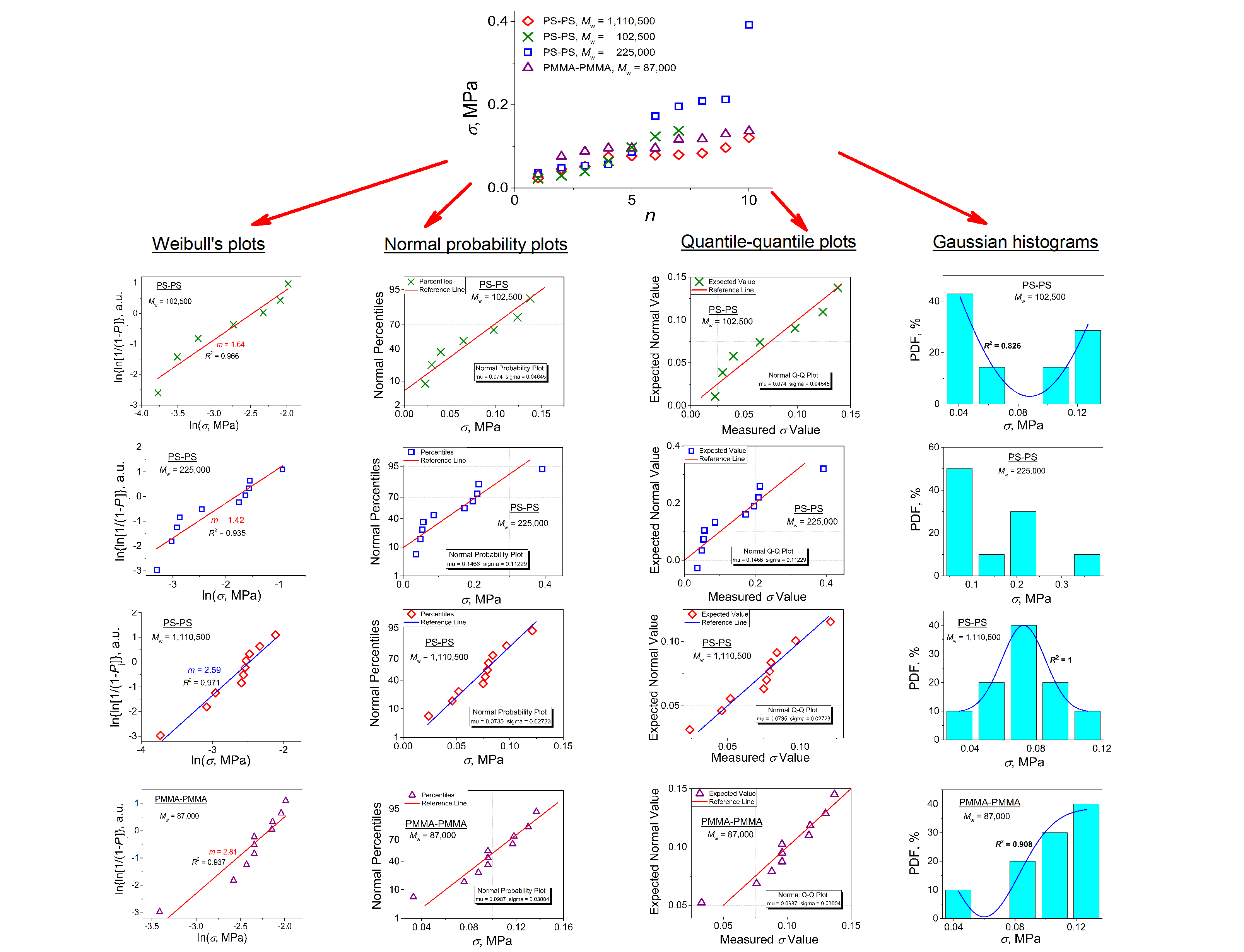
Now, turn to the statistical analysis of the four σ data sets presented in Fig. 2. First, their conformity to Eq. (1) in the framework of Weibull’s model was examined by replotting them as lnln[1/(1 − Рj)] vs lnσ and applying linear regression analysis. The results of this procedure are presented in Fig. 3. In general, the data points plotted in Weibull coordinates “lnln[1/(1 − Рj)] − lnσ” represent linear curves characterized by rather high root mean square deviations R2 of 0.936 to 0.971. These observations indicate that the experimental data obey Weibull statistics. Among the three PSs investigated, the smallest value of the Weibull’s modulus (m = 1.42) is characteristic of the polydisperse PS1 (see Fig. 3b) compared to those for the near-monodisperse PS2 (m = 1.64) and PS3 (m = 2.59) (see Fig. 3a and Fig. 3c, respectively). This means that the data scatter for the former is broader than that for the latter. This behavior may be explained by the fact that the interdiffusion process in the polydisperse polymer with a larger variation in Lchain (PS1) should be less uniform than that for the two monodisperse polymers, each of which has roughly constant Lchain value (PS2 and PS3).
Figure 3 Weibull plots for the data presented in Fig. 2 for AJs (a) PS1-PS1, (b) PS2-PS2, (c) PS3-PS3, and (d) PMMA-PMMA. The solid lines are linear fits to the data points.
The values m = 1.64 and 2.59 reported in Fig. 3 for the weak PS2-PS2 (at T = Tg − 81°C) and PS3-PS3 (at T = Tg − 82°C) interfaces (σ = 0.02−0.12 MPa), respectively, are close to those reported recently [41] for the PS2-PS2 (m = 2.40) and PS3-PS3 (m = 1.89) interfaces but characterized by a greater adhesion strength by a factor of five (σ = 0.1−0.6 MPa) due to its development at a markedly higher T = Tgbulk − 33°C. Hence, the substantial changes in T by 50°C and in σ by a factor of five had almost no impact on the Weibull distribution behavior of the adhesion strength of these two PSs. Comparable m values have been reported for the following weak polymer‒polymer interfaces self-bonded at T < Tg: m = 0.54−2.78 for the PS-its blend with poly(2,6-dimethyl-1,4-phenylene oxide) interface [22] and m = 1.11−2.14 for the PS-PS, PMMA-PMMA, and PS-PMMA interfaces [23]. However, these m values are markedly smaller than those for m = 3−17 for the weak (σ = 0.1−0.6 MPa) compatible PET-PET [21] and incompatible PS-PET interfaces (m = 3−10) [25] self-bonded at T > Tg [21] and at both T > Tg and T < Tg [25]. Therefore, it may be concluded that the highest m values (or the narrowest data scatter) are estimated for interfaces when at least one surface in contact is the PET surface.
Higher values of m = 7.7−45.3 have been reported for high-strength (σ = 0.2−6 GPa) fibers of polypropylene, polyamide 6, and ultrahigh-molecular weight polyethylene [33, 59]. Nevertheless, this m interval overlaps with that of m = 3−17 for PET interfaces, despite the tremendous difference (by three to four orders of magnitude) between the adhesion strength of the weak polymer-polymer interfaces and the tensile strength of the high-performance polymer fibers. This behavior may be explained by the fact that these two sample types, low-strength AJs and high-strength fibers are similar from the point of view of being both quasibrittle.
We turn now to the question of the conformity of the data sets reported in Fig. 2 to the normal distribution by considering them, first, as the normal probability and quantile–quantile plots in Fig. 4 and Fig. 5, respectively. As a result of these two procedures, one obtains the standard deviation (SD) and the arithmetic mean value (σav). The values of SD and σav were calculated using either the NP or Q−Q plots and were the same for each of the interfaces investigated. Hence, any of these plot types can be chosen arbitrarily to perform such a statistical analysis.
Figure 5 Normal Q–Q plots for AJs (a) PS1-PS1, (b) PS2-PS2, (c) PS3-PS3, and (d) PMMA-PMMA
Let us estimate a ‘measure’ of the reduced data scatter, i.e., the SD value is reduced to σav. This approach gives one an opportunity to correctly compare the data scatter for the samples with strongly differing values of SD and σav and to operate with a dimensionless parameter. The results of the analysis carried out above are shown in Table 2. Among the three PSs investigated, the smallest and largest values of SD/σav were estimated for PS3 (0.370) and PS1 (0.766), indicating the narrowest and the broadest reduced data scatter, respectively. PMMA demonstrated the narrowest data scatter (SD/σav = 0.304) compared to those for the three PSs investigated. The same trend follows from the Weibull analysis (see the m values in Table 2) since an increase in m means a decrease in the data scatter. Hence, by comparing SD/σav with 1/m and by normalizing SD/σav by 1/m, one may expect some correlation between these two different statistical characteristics and their variation. It is interesting to note that the results of this procedure give values of (SD/σav)/(1/m), which are close to 1, especially for PSs (see the last line in Table 2). Therefore, this parameter may be treated as a universal constant representing the material data scatter. In fact, these two statistical characteristics, SD/σav and 1/m, obtained using different statistical methods are close and can be used for their direct mutual recalculation as SD/σav ≈ 1/m.
To investigate the issue of normality in more detail, we analyzed the data sets received using the six widely used normality tests listed previously. The results obtained with the help of these procedures are shown in Table 3 and Table 4.
Table 2
Statistical parameters at T = 24°C calculated from graphical methods
|
Polymer
Statistical parameter
|
PS1
|
PS2
|
PS3
|
PMMA
|
|
σav, MPa
SD, MPa
SD/σav
Equation (2)
Fitting reliability (R2)
σ0, MPa
σ0/σav
Weibull’s modulus, m
1/m
(SD/σav)/(1/m)
|
0.14660
0.11229
0.766
y = 2.56 + 1.42x
0.935
0.16465
1.12
1.42
0.704
1.09
|
0.07400
0.04645
0.628
y = 4.05 + 1.64x
0.966
0.08449
1.14
1.64
0.610
1.03
|
0.07350
0.02723
0.370
y = 6.41 + 2.59x
0.971
0.08404
1.14
2.59
0.386
0.959
|
0.09870
0.03004
0.304
y = 10.26 + 4.66x
0.974
0.11046
1.12
4.66
0.356
0.854
|
Table 3
Statistical parameters of the lap-shear strength distribution at RT estimated for the PS-PS and PMMA-PMMA interfaces using five tests for normality
|
Polymer
|
Test type
|
Statistic
|
p value
|
Decision at level 5%*
|
|
PS1
PS2
PS3
PMMA
|
Shapiro–Wilk
|
0.85455
0.90643
0.95842
0.91994
|
0.06579
0.37171
0.76772
0.33645
|
+
+
+
+
|
|
PS1
PS2
PS3
PMMA
|
Lilliefors
|
0.20529
0.19647
0.22196
0.16419
|
0.20000
0.20000
0.16132
0.20000
|
+
+
+
+
|
|
PS1
PS2
PS3
PMMA
|
Kolmogorov–Smirnov
|
0.20529
0.19647
0.22196
0.16419
|
0.75831
1.00000
0.65164
1.00000
|
+
+
+
+
|
|
PS1
PS2
PS3
PMMA
|
Anderson–Darling
|
0.59584
0.31330
0.32945
0.37195
|
0.08789
0.44565
0.44492
0.34681
|
+
+
+
+
|
|
D’Agostino–K squared:
|
|
PS1
PS2
PS3
PMMA
|
Omnibus
Skewness
Kurtosis
Kurtosis
Omnibus
Skewness
Kurtosis
Omnibus
Skewness
Kurtosis
|
3.75256
1.64476
1.0234
−1.34969
0.42441
−0.31339
0.57114
3.73101
−1.47967
1.24161
|
0.15316
0.10002
0.30612
0.17711
0.80880
0.75399
0.56791
0.15482
0.13896
0.21438
|
+
+
+
+
+
+
+
+
+
+
|
| * “+” in column 5 means “cannot reject normality” |
Table 4
Statistical parameters of the lap-shear strength distribution for PS-PS interfaces and PMMA-PMMA estimated using the Chen–Shapiro test for normality
|
Polymer
|
Statistic
|
10% critical value
|
5% critical value
|
Decision at level 5%*
|
|
PS1
PS3
PMMA
|
0.05358
−0.13752
−0.06930
|
0.01981
0.01981
0.01981
|
0.06668
0.06668
0.06668
|
+
+
+
|
| * “+” in column 5 means “cannot reject normality” |
The result “cannot reject normality” was obtained for all the datasets analyzed. Considering that the test rejects the null hypothesis of normality when the p value is less than or equal to 0.05 [42 − 53], formally, all the p values listed in Table 3, which are larger than 0.05, meet this requirement. Therefore, the statistical distribution of each of these four σ datasets is expected to have the shape of a bell curve. To test this hypothesis, we compare the results of these tests for normality with the histograms of the probability density function (PDF) as a function of σ constructed for the four polymers investigated in Figs. 6a, 6b, 6c, and 6d. Based on these results, one may conclude that, formally, Gaussian fitting works well for all four histograms considered. However, the classical bell-shaped curve is observed only for PS3, which has the largest Mn ≈ 103 kg/mol (see Fig. 6c), while the inverted Gaussian curves with bimodal distributions with the minimum in the center were obtained for PS1, PS2, and, to a lesser extent, PMMA. In particular, the majority of the data points (∼45%) for PS1 and PS2, with markedly lower Mn values < 102 kg/mol, fall within the interval of smallest strengths (see Fig. 6a and Fig. 6b). In contrast, they are concentrated in the histogram center for PS3 (see Fig. 6c), i.e., for the polymer with the longest chains but with the smallest chain-end concentration; on the other hand, they are longer or smaller by an order of magnitude compared to the corresponding values of Lchain and Cends for the other polymers. The PMMA strength distribution is concentrated at higher strengths. Although this histogram can be formally fitted with a Gaussian function with R2 = 0.908, it cannot be taken for that to conform correctly to the normal inverted distribution.
Therefore, the analysis of the normal distribution behavior revealed its dependence on three molecular factors: Mn, Mw/Mn, and the chemical structure of the polymer. These results may be rationalized as follows.
Although the p values estimated in the normality tests are always greater than p = 0.05 and agree with the null hypothesis of normality, some of the p values for PS1 are comparable to this p value, which does not support the observation of a bell curve in the following cases: the Shapiro–Wilk test (p = 0.06579), the Anderson–Darling test (p = 0.08789), and the D’Agostino–K-squared test (p = 0.10002). In contrast, the p values for PS3 estimated in these tests are markedly greater: p = 0.76772 (the Shapiro–Wilk test), p = 0.44492 (the Anderson–Darling test), and p = 0.8088 and 0.75399 (the D’Agostino–K squared tests), which are in good agreement with the observation of the bell curve for PS3. As far as the Kolmogorov–Smirnov and Lilliefors tests are concerned, they give rather similar p values for the four polymers investigated. However, the smallest p values were obtained for PS3 (0.65164 and 0.16132), which is quite surprising since the classical bell curve was observed for this polymer only. Therefore, these two tests seem to be inappropriate for properly characterizing the distribution of the interfacial strength at weak polymer-polymer interfaces. Thus, not all of the normality tests employed can correctly estimate the conformity to the normal distribution received in the graphical analysis. The best fitting results for all four interfaces considered were obtained with the help of Weibull’s model, which is not surprising because of the brittleness of all these interfaces.
Figure 6 Histograms of PDF vs σ for AJs (a) PS1-PS1, (b) PS2-PS2, (c) PS3-PS3, and (d) PMMA-PMMA; Gaussian fits are shown with solid lines
Among the three PSs investigated, the largest differences in the lap-shear strength distribution behavior were found for the polydisperse PS1 (Mw/Mn = 3) and near-monodisperse PS3 (Mw/Mn = 1.15): both the Weibull and Gaussian fitting results were more correct for PS3 than for PS1, while the σ values for PS1 were greater than those for PS3. These differences can be caused by, along with Mw/Mn, Cends, and Lchain considered previously, molecular factors such as (i) the total number of the statistical segments per chain Ntotal = Nru/c∞, where Nru is the number of repeat units per chain, which is equal to Mn/Mru; (ii) the number of chain end segments (Nends = 2); and (iii) the number of central chain portion segments Ncenter = Ntotal − Nends. Using Mru = 104 g/mol and c∞ = 10 for PS [54, 55], one obtains Ntotal = 72 and 928 for PS1 and PS3, respectively; hence, Ncenter = 70 and 926 for PS1 and PS3, respectively. Therefore, the fractions of Nends and Ncenter in Ntotal are Nends/Ntotal = 0.028 and 0.002, respectively, while Ncenter/Ntotal = 0.972 and 0.998 for PS1 and PS3, respectively. Therefore, the 0.2% fraction of the chain-end segments in PS3 is negligible and statistically insignificant, while the 2.8% fraction in PS1 can notably contribute to the self-healing process at the interface; in particular, the higher mobility of the chain ends results in higher strength values for PS1. Nevertheless, the major contribution to the σ value should be provided by the segments of the central chain portions since their fraction of 97.2% is very large. Therefore, as a combined result of these two contributions, one observes the inverted Gaussian σ distribution for PS1. Additionally, an additional contribution to this behavior may be caused by the negative effect of a greater concentration of chain ends, which represent ‘structural defects’, in contrast to their positive effect on the development of a greater adhesion strength due to their greater mobility. In the case of PS3, the chain-end contribution may be neglected due to the small value of Nends/Ntotal = 0.2%. For this polymer, an almost total σ of 99.8% is attributed to the central chain portions. Therefore, the strength evolution process should be more uniform statistically, on the one hand, but the values of the developed strength should be smaller, on the other hand, as is actually observed in Fig. 6c.
Notably, long-range cooperative segmental motions involving segments of several neighboring chains are activated only at T > Tg and frozen at T < Tg [5, 54]. Only at T > Tg can the reptation mechanism consisting of the translation-rotation displacement of an individual chain along its backbone in a snake-like manner within a hypothetical tube in an entangled medium, i.e., for polymers with M > Ment, be realized across the interface. Therefore, the process of lap-shear strength development at the PS-PS and PMMA-PMMA interfaces at room temperature proceeded through the viscoelastic interface layer at T > Tginterface, allowing the chain segments to cross the interface between the two contacting polymer specimens and create new physical links on the interface counterside, thus providing mechanically resistant autoadhesion. In turn, the validity of this molecular mechanism indicates that the outermost surface layer prior to contact was in the viscoelastic, not glassy, physical state (at T > Tgs) at T = 24°C, even at T = Tg − 85°C. This marked decrease in Tgs with respect to Tg(bulk) is due to the significantly longer contact times (up to 2 months) used in the present work than those used previously (4 days at most) [2] when the PS autoadhesion has also been observed below Tg but at a higher Talowest = Tg − 67°C. This decrease in the PS Tgs with respect to the PS Tg with an increase in t is one more valid argument in favor of the relaxation nature of the glass transition phenomenon at polymer surfaces since Talowest would not be dependent on T and t in the case of its thermodynamic nature and its correspondence to T2.
Let us now determine how an increase in T from its extremely low T for such processes (T = 24°C) to T = 64 (PS1), 72 (PS2), 73 (PS3), and 74°C (PMMA), which correspond to T = Tg – 33°C for all the three PSs investigated, and to the rather close T = Tg – 35°C for PMMA can impact the statistical behavior of the adhesion strength. The results of the measurements for the AJs self-bonded at those temperatures for 24 h are presented in Fig. 7a. By applying the same procedures used for the statistical analysis as previously described, one obtains the results presented in Fig. 7b; Figs. 8a, 8b, 8c, and 8d; Table 5, Table 6, and Table 7; and Figs. 9a, 9b, 9c, and 9d.
Table 5
Statistical parameters at T = Tg – 33°C and t = 24 h calculated from graphical methods
|
Polymer
Statistical parameter
|
PS1
|
PS2
|
PS3
|
PMMA
|
|
σav, MPa
SD, MPa
SD/σav
Equation (2)
Weibull’s fitting reliability (R2)
σ0, MPa
σ0/σav
Weibull’s modulus, m
1/m
(SD/σav)/(1/m)
|
0.39250
0.19081
0.486
y = 1.37 + 1.74x
0.971
0.4548
1.16
1.74
0.575
0.845
|
0.26945
0.13132
0.487
y = 2.86 + 2.40x
0.982
0.3035
1.13
2.40
0.417
1.17
|
0.14411
0.07739
0.537
y = 3.57 + 1.97x
0.988
0.1631
1.13
1.97
0.508
1.06
|
0.24840
0.06278
0.253
y = 5.67 + 4.37x
0.953
0.2730
1.10
4.37
0.229
1.10
|
Table 6
Statistical parameters of the lap-shear strength distribution at T = Tg – 33°C and t = 24 h estimated for the PS-PS and PMMA-PMMA interfaces using five tests for normality
|
Polymer
|
Test type
|
Statistic
|
p value
|
Decision at level 5%*
|
|
PS1
PS2
PS3
PMMA
|
Shapiro–Wilk
|
0.95130
0.92935
0.93979
0.90315
|
0.44580
0.15004
0.26140
0.04727
|
+
+
+
−
|
|
PS1
PS2
PS3
PMMA
|
Lilliefors
|
0.11817
0.15347
0.15788
0.17859
|
0.20000
0.20000
0.20000
0.09427
|
+
+
+
+
|
|
PS1
PS2
PS3
PMMA
|
Kolmogorov–Smirnov
|
0.11817
0.15347
0.15788
0.17859
|
1.00000
0.70769
0.70223
0.49805
|
+
+
+
+
|
|
PS1
PS2
PS3
PMMA
|
Anderson–Darling
|
0.32118
0.49761
0.41675
0.71855
|
0.50507
0.18727
0.29844
0.05105
|
+
+
+
+
|
|
D’Agostino–K squared:
|
|
PS1
PS2
PS3
PMMA
|
Omnibus
Skewness
Kurtosis
Omnibus
Skewness
Kurtosis
Omnibus
Skewness
Kurtosis
Omnibus
Skewness
Kurtosis
|
1.03477
−0.53671
−0.86412
1.95367
1.36904
−0.28178
1.94532
0.79625
−1.14512
6.01671
−0.54627
−2.3913
|
0.59608
0.59147
0.38752
0.37650
0.17099
0.77811
0.37808
0.42589
0.25216
0.04937
0.58488
0.01679
|
+
+
+
+
+
+
+
+
+
−
+
−
|
| * “+” in column 5 means “cannot reject normality” |
Table 7
Statistical parameters of the lap-shear strength distribution at T = Tg – 33°C and t = 24 h for the PS-PS interfaces and PMMA-PMMA estimated using the Chen–Shapiro test for normality
|
Polymer
|
Statistic
|
10% critical value
|
5% critical value
|
Decision at level 5%*
|
|
PS1
PS2
PS3
PMMA
|
−0.07000
−0.00868
−0.03627
0.06218
|
0.01484
0.01371
0.01427
0.01371
|
0.05362
0.05109
0.05232
0.05109
|
+
+
+
−
|
| * “+” in column 5 means “cannot reject normality” |
Figure 9 Histograms of PDF vs σ for AJs (a) PS1-PS1, (b) PS2-PS2, (c) PS3-PS3, and (d) PMMA-PMMA; the Gaussian fit is shown with the solid line
It follows from Fig. 7b and Table 5 that Weibull’s model works properly for the four interfaces investigated since R2 ≥ 0.953 or even > 0.97 for PSs. The values of Weibull’s modulus are close to the corresponding values reported in Table 2 for room temperature, and the average strength values estimated from both the probability plots (σav) and Weibull’s analysis (σ0) are close. In addition, the values of (SD/σav)/(1/m) collected in Table 5 characterize the relationship between the reduced statistical parameters estimated using two different approaches for a markedly higher T = 64−74 °C were close to 1, as in the case of T = 24°C (see Table 2). This finding suggests that the (SD/σav)/(1/m) ratio introduced by us as a link between two different statistical approaches is a statistical constant of a universal nature. It can be used for mutual recalculation of SD/σav and 1/m since the (SD/σav)/(1/m) ratio is close to 1.
The p values for the three PSs investigated calculated in the tests for normality (see Table 6) are greater than 0.05, indicating that the probability density distribution curves should have a bell shape. In contrast, some of the p values for PMMA were close to or less than 0.05, which suggests that a bell-shaped PDF (σ) curve is not expected for this polymer. However, as follows from Figs. 9a, 9b, 9c, and 9d, contrary to expectations, the (inverse) bell curve is observed for PMMA only (see Fig. 9d). For PS1, PS2, and PS3 (see Figs. 9a, 9b, and 9c), the bell curve cannot be drawn reliably since the σ distributions for all three PSs investigated have a random character. This behavior differs from that at T = 24°C. Therefore, as self-bonding progresses and the strength increases, the Gaussian model becomes less appropriate.