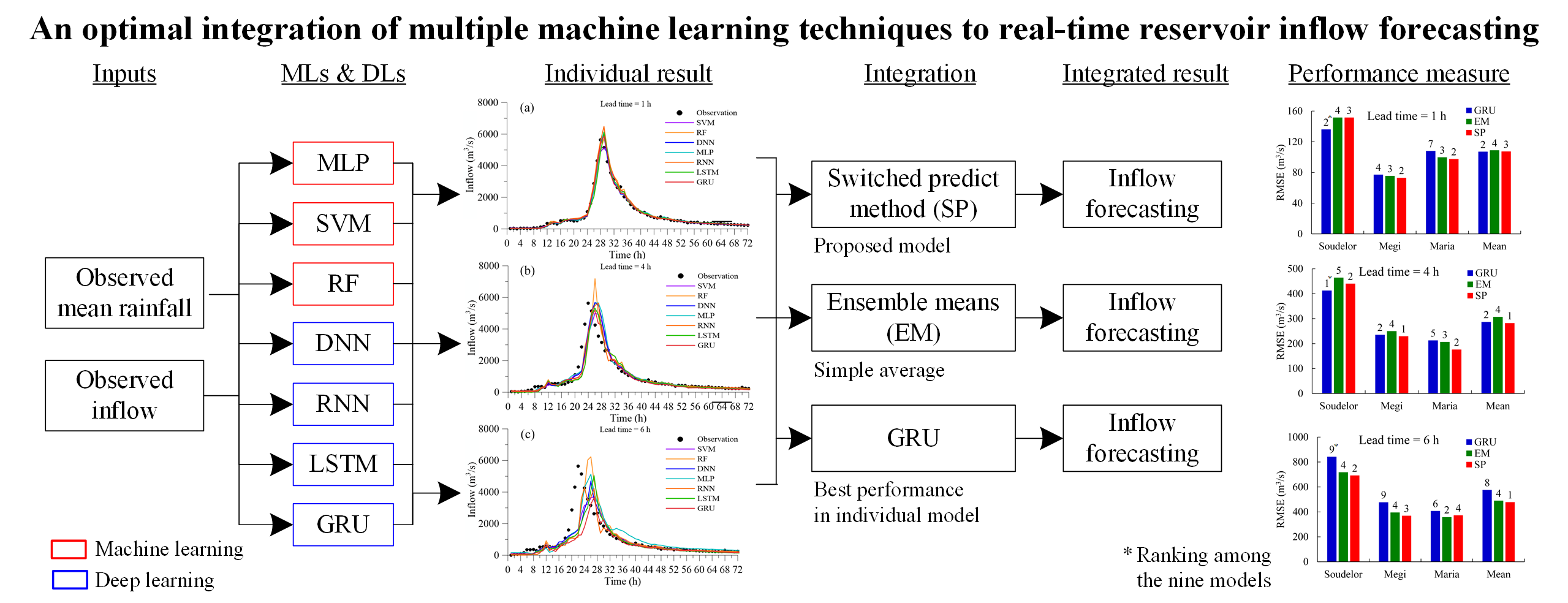
A reservoir inflow forecasting system represents a crucial technique in reservoir operation and disaster prevention, particularly in areas where the primary water source derives from typhoon events. This includes the study area of the current research, i.e., the Shimen Reservoir (Taiwan). Effectively depositing short and high-intensity rainfall and avoiding disaster losses present significant challenges in this regard. However, the high variability and uncertainty of such rainfall events make them difficult to forecast using traditional physical-based models, which require too many calculations for application in real-time disaster forecasting. Accordingly, in this study, seven machine learning (ML) algorithms, including three conventional ML and four deep learning algorithms, were compared to derive their effectiveness for reservoir inflow forecasting in extreme weather events. The forecasting lead-times were set to 1, 4, and 6-h, representing short, medium, and long-term forecasting, respectively. Moreover, to ensure the stability and credibility of the models, two types of integrated approaches, ensemble means and switched prediction method (SP) were also employed. The results showed that although an optimal algorithm could be selected for the short, medium, and long-term, individual algorithms did not always perform well in all events. Nonetheless, the integrated approaches can effectively combine the advantages of all the included algorithms and generate more accurate and stable forecasting results, particularly when using SP, which was involved in the top three performances among all typhoon examples and indicated the best average performance. Accordingly, when using a single forecasting algorithm, gated recurrent unit, a type of transformed recurrent neural network, will yield the best performance. Furthermore, integrated forecasts, particularly involving SP, can effectively improve the accuracy and stability of forecasts to render a model more applicable to an actual situation.
Research Article
An Optimal Integration of Multiple Machine Learning Techniques to Real-Time Reservoir Inflow Forecasting
https://doi.org/10.21203/rs.3.rs-599274/v1
This work is licensed under a CC BY 4.0 License
You are reading this latest preprint version
Reservoir Inflow Forecasting
Ensemble Forecasting
Machine Learning
Deep Learning
Switched Prediction
In recent years, climate change has received significant attention due to global warming, which has led to the rising sea levels and a higher frequency of extreme weather events. Water resource management and disaster prevention have become vital subjects. Based on the location and climate of Taiwan, the area experienced an average of three to four typhoons annually from 1911 to 2019. The average annual rainfall of Taiwan is 2,500 mm, 2.6 times higher than the average global precipitation. Despite this abundant rainfall during typhoon events, reservoirs in Taiwan are unable to store these large water resources, which are accumulated within short-term rainfall durations. As a result, rather than serving as a resource, excessive rainfall may cause disasters such as flooding and landslide. To prevent the loss of human life and property, a sophisticated management system and erudite operation of reservoirs are necessary.
Reservoir inflow forecasts are crucial techniques for the management and operation of water resources. Especially for Taiwan, which is shaped long and narrow, where reservoir management will highly impact both the water supply for daily living and industrial use. As such, an accurate reservoir inflow forecasting model will be indispensable for managing the water supply systems in Taiwan. As previously noted, researchers have attempted to construct inflow forecasting models using empirical and conceptual methods. Young et al. (2015) used the inflow, which was known as reservoir inflow, forecasted by the hydrologic modeling system (HEC-HMS) as an input for artificial neural networks (ANNs) to forecast future inflow over a 6-h lead-time. In the same year, the researchers employed the inflow forecasted by HEC-HMS using a genetic algorithm neural network and adaptive-network-based fuzzy inference system to create inflow forecasting models, with a 6-h lead-time. Noori and Kalin (2016) used the soil and water assessment tool to simulate the base flow, surface runoff, and interflow as input factors of ANNs to forecast a 24-h lead-time inflow. Young et al. (2017) simulated the inflow through HEC-HMS and used forecasting inflow as the input factors for the support vector machine (SVM) model to forecast a 6-h lead-time inflow. Ren et al. (2018) used ten atmospheric factors selected from JRA-55, and simulated the snowmelt–rainfall-produced inflow generated by the Hydrologiska Byråns Vattenbalansavedlning (HBV) model as the inputs of a Bayesian neural network; the least-squares model (SVM) was used to forecast monthly inflow.
Because of the typhoon events that are often present as nonlinear complex trends, machine learning (ML) that can effectively handle nonlinear features was adopted in this study. The ML used in this study can be grouped into two categories, i.e., the conventional ML and deep learning (DL), the latter having received significant attention in recent years. Conventional ML such as SVM and random forest (RF) models has been popular for several decades in numerous fields including hydrological forecasts. Yu et al. (2009) constructed SVMs based on two different input groups to forecast water levels. Kuo (2014) used RF to create 1–3-h lead-time water-level forecasting models; here, RF results indicated the presence of a lag time and an error in peak-value estimation as the lead-time became longer. With the recent rapid development of DL, ever more studies indicate that it can effectively deal with complex features hidden in big data. In 2012, AlexNet (Krizhevsky et al., 2017), a pioneering DL neural network, won first prize in the ImageNet Large Scale Visual Recognition Challenge. Following on, many researchers from a broad range of fields have engaged in the development of different types of DL. Matthwe and Fergus (2013) created ZFNet, a deep learning structure that employs multilayer inverse convolution networks to visualize the changing process of features while training networks. Using ZFNet, users can realize the potential problems in models in real time, discuss how local features could affect classification results, and generalize the types of features indicating a higher correlation with each classified group. Szegedy et al. (2014) presented GoogLeNet, a convolutional neural network (CNN) that deepens networks and reduces the number of connections between each layer. Employing this model, Szegedy et al. used a convolution kernel to deliver the weights and a multi-channel approach to reduce model complexity. This design renders networks more powerful without increasing parameters that may lead to training difficulty.
As noted above, most DL algorithms have been used in image recognition over the past number of years. With many studies showing the advantages of DL algorithm, ever more researchers from different fields have adopted such models to overcome various problems. In the field of meteorology and hydrology, Tao et al. (2016) constructed the stacked denoising autoencoder in four layers and comprising 1,000 nodes to analyze \(15\times 15\) pixel cloud images, and subsequently used these images to forecast precipitation. Their results showed that precipitation forecasting combining DL techniques were between 33–43% more accurate than traditional precipitation estimations from remotely sensed information using an ANN cloud classification system. Song et al. (2016) used soil surface temperature and leaf area index as inputs to develop DL that could effectively forecast soil surface humidity. Bai et al. (2016) used non-recurrent deep backpropagation networks to forecast pinpoint inflow for the Three Gorges Dam (TGD) reservoir (China). Their results showed that DL could accurately forecast inflow and effectively handle multi-dimensional problems and complex features in the engineering field. Furthermore, their results indicated models constructed using Fourier transform input data are more accurate than those created by data without preprocessing. Liang et al. (2018) used long short-term memory (LSTM) to analyze water-level variations in Dongting Lake (China) and discussed the impact of TGD on the lake. Their results showed that models constructed with LSTM had observably higher accuracy than conventional SVM models. The experiment also showed that the TGD could effectively alleviate the disaster during extreme events no matter flood or drought. Zhang et al. (2018) selected LSTM and a gated recurrent network (GRU) to forecast water levels in a sewage treatment facility. Their results indicated that both LSTM and GRU could effectively improve forecasting accuracy. In their study, GRU was somewhat more accurate than LSTMs because the input data employed in the research were comparatively less. In general, DL can effectively ameliorate the shortages of traditional time-series statistical methods. Kratzert et al. (2018) constructed streamflow forecasting models for hundreds of American watersheds and also employed these forecasting results in the soil moisture calculating models for Sacramento, California. According to the results of this study, LSTM could capture the small features hidden within the physical parameters. A DL model cannot be properly trained using only a single set of watershed data; data from different watersheds should be used. Once the parameters for DL models have been established, and using sufficient training data, DL models will be able to improve the forecasting performance.
As noted above, in the field of hydrology, few studies have adopted DL methods, with the bulk of studies preferring image recognition methods to classify cloud images and inundation maps. Alternatively, improved recurrent neural networks (RNNs) such as LSTM and GRU have also been used to forecast the time-series data. In the current study, we selected three conventional ML methods, i.e., SVM, RF, and multilayer perceptron (MLP). In addition, the DL models used in this study were divided into conventional and recurrent deep neural networks (DNNs). The conventional group included DNNs, and the recurrent group included RNN, LSTM, and GRU. In the first section of this study, we selected these seven models to establish 1–6-h lead-time reservoir inflow forecasting models. To more objectively evaluate the performance of algorithms, we used six performance measures to determine the best reservoir inflow forecasting model.
Discussions of the first part regarding performance of individual model will focus on three phases. First, the conventional MLP will be compared with DNN to derive the differences between conventional ML and DL. Second, RNN and GRU will be compared with LSTM to explore how gate units (included in LSTM and GRU) influence prediction accuracy. Third, seven algorithms will be compared in a unified manner, and their pros and cons will be discussed according to 1, 4, and 6-h lead-time forecasting scenarios for typhoons. The results showed that although the single best algorithm could be determined by averaging the performance measures calculated from all events, this result did not necessarily ensure that the (comparatively) best algorithm could perform stably and efficiently in all typhoon cases. Hence, two integrated methods, ensemble means (EM) and switched prediction (SP), are used in this study to integrate the results of seven algorithms as hybrid forecasting approaches. The results showed that hybrid forecasting effectively increased the forecasting stability, and forecasting results using EM (with the principle to average the results obtained from all seven algorithms) could steadily exceed the performance of half of using individual model scenarios in all typhoon examples. Moreover, the integrated results generated by SP achieved the top three performances among all seven algorithms and performed the best in case of all typhoon examples on average. This indicates that the integrated forecasting approach is more reliable and can be used in actual reservoir operations during extreme events.
Shimen Reservoir, located in northern Taiwan, was once the largest reservoir in the Far East region. As a multi-objective hydraulic structure, the reservoir is involved in irrigation, power generation, water supply, and flood control, and even serves as a sightseeing destination. The length and total area of the reservoir are approximately 16.5 km and 8 km2, respectively. The Shimen Reservoir catchment area is 763.4 km2. Total reservoir and effective capacities are 309 and 209 billion m3. Based on the position of the reservoir, rainfall primarily derives from monsoons and typhoons. From 1911 to 2019, on average, 3.6 typhoons crossed through the area yearly, delivering more than 2,000 mm of annual average precipitation. Figure 1 shows the study area adopted in this study. Eight rainfall (or meteorological) stations’ rainfall data from 2004 to 2018 were collected to construct the reservoir inflow forecasting model. The model was considered for operational and warning uses in extreme events, in which the training and test datasets would be selected in an event-oriented manner. Accordingly, 18 typhoons (with intact and high-quality data) were adopted as shown in Table 1. Among these events, the proportion of training and test datasets was set to 13:5 in this study. The data were collected by the Water Resources Agency (WRA) in Taiwan, and the time interval for raw data was approximately 1 h.
| Number | Event | Date (yyyy/mm/dd) | Duration (h) | Max. hourly rainfall (mm) | Peak inflow (m3/s) |
|---|---|---|---|---|---|
| Training events | |||||
| 1 | Acre | 2004/8/23 | 96 | 53.4 | 8593.9 |
| 2 | Krosa | 2007/10/5 | 144 | 40.5 | 5300.4 |
| 3 | Kalmaegi | 2008/7/16 | 57 | 8.8 | 205.7 |
| 4 | Fung-Wong | 2008/7/26 | 89 | 17.2 | 2039.8 |
| 5 | Sinlaku | 2008/9/11 | 313 | 30.8 | 3446.9 |
| 6 | Jangmi | 2008/9/26 | 150 | 31.4 | 3292 |
| 7 | Morakot | 2009/8/6 | 120 | 46.8 | 1837.5 |
| 8 | Fanapi | 2010/9/19 | 72 | 21.9 | 1056.2 |
| 9 | Saola | 2012/7/30 | 167 | 45.9 | 5385.1 |
| 10 | Trami | 2013/8/20 | 156 | 27.8 | 2410.1 |
| 11 | Soulik | 2013/7/11 | 135 | 38.7 | 5457.9 |
| 12 | Dujuan | 2015/9/29 | 106 | 36.4 | 3802.5 |
| 13 | Meranti | 2016/9/13 | 94 | 6.8 | 451.8 |
| Test events | |||||
| 14 | Soudelor | 2015/8/6 | 73 | 47.4 | 5634.1 |
| 15 | Nepartak | 2016/7/7 | 85 | 3.8 | 259.1 |
| 16 | Malakas | 2016/9/16 | 94 | 13.1 | 601 |
| 17 | Megi | 2016/9/26 | 94 | 41 | 4267.6 |
| 18 | Maria | 2018/7/9 | 23 | 23.2 | 1702.1 |
In this section, we introduce the algorithms used in this study. Conventional ML algorithms such as SVM, RF, and MLP are described in Sect. 3.1. These models were created using the Scikit-learn (v. 0.22.1) software package in Python. The DL algorithms, DNN, RNN, LSTM, and GRU, are presented in Sect. 3.2. These models were created using Tensorflow (v. 2.1) and Keras (Google). The hyperparameters of all algorithms were determined using the grid-search method. Details of the grid-search method can be found in Lerman (1980). The SP algorithm is illustrated in Sect. 3.3. In Sect. 3.4, the research process has been explained.
3.1 Machine learning
3.1.1 Support vector machine
As a powerful supervised learning algorithm, SVM was created by Vapnik (1995) to overcome the challenges of problems identified in the early 1990s. In 1995, SVM was used to address a regressive problem and showed exemplary performance. There are two main advantages of using SVM. First, the structural risk minimization adopted by the SVM can effectively reduce the loss of function without increasing the structural complexity of a model, allowing it to balance both its accuracy and computational speed. Additionally, solutions related to the structure and weights in the SVM can be simplified as a quadratic programming problem, which can be resolved using a standardized process. In recent years, the SVM was applied to several fields and performed with extremely high accuracy, regardless of the classification or regression applications involved. More details about the principles of the SVM can be found in the literature (Vapnik and Cortes, 1995; Cristianini and Shawe-Taylor, 2000).
3.1.2 Random forest
Created by Breiman (2001), RF is a powerful ensemble-learning ML algorithm that can be constructed using multiple decision trees. Based on the principles of RF, this algorithm has several advantages. First, in contrast to conventional ML algorithms, such as SVM and backpropagation networks, RF can effectively handle large amounts of input variables without with the need to address dilemmas about data dependency and overfitting. Second, the randomness involved in bootstrapping contributes to the stronger ability of anti-noise from raw data. Furthermore, the large number of decision trees in RF also gives rise to its highly suitable ability for nonlinear functioning. Based on these advantages, RF has become one of the most popular ML algorithms for use in classification and regression; it is widely adopted in research and has even been used in competitions hosted by Kaggle, one of the most famous data science community. More details about RF can be found in Liaw and Wiener (2002).
3.1.3 Multilayer perceptron
Proposed by Rumelhart et al. in 1986, the MLP is a classic backpropagation neural network that can be constructed using three types of layers, i.e., input, hidden, and output layers. As a supervised learning model, the weight correction algorithm used in MLP is backpropagation. To distinguish it from the use of a DNN model, the activation function used in MLP does not include a relatively novel function (e.g., rectified linear unit [ReLU]). The number of hidden layers was also restricted to one. Because MLP was used for conducting regression in this study, the loss function, mean square error was adopted, and the optimization approach was classic stochastic gradient descent.
3.2 Deep learning
In contrast to conventional ML algorithms, the key concept of DL is to learn representation from raw data without the need for complicated model designing and data preprocessing. In the 1980s, data scientists were inspired by how the neurons work in living organisms, which inspired the creation of ANNs. As heuristic algorithms, ANNs have rapidly evolved into several different structures, such as RNNs and CNNs. However, at the time, restricted by hardware operation capabilities, these creative networks were unable to achieve breakthrough performances. By continuously improving the performance of hardware components post 2000, these algorithms, combined with DL, were gradually applied to computer vision and natural language processing.
In this study, to efficiently forecast 1–6-h lead-time reservoir inflow (which were considered as standard time-series data), four DL algorithms that are commonly used to manage time-series problems were employed. Next, we introduced the DNN in Sect. 3.2.1, the RNN in Sect. 3.2.2, the LSTM in Sect. 3.2.3, and the GRU in Sect. 3.2.4.
3.2.1 Deep neural networks
Hinton first proposed DNNs in 2006, which applied the restricted Boltzmann machine (RBM) ANN to initialize parameters and successfully overcome the optimization problem due to backpropagation. In addition to the RBM, several innovations occurred between the development of DNN and MLP models. First, traditional MLP in the 1980s typically had no more than three hidden layers. Contrastingly, networks nowadays almost always have more than three hidden layers as shown in Fig. 2(a). Additionally, when applied to regression problems, the ReLU function is used to replace the most commonly used activation function, i.e., the sigmoid. Novel parameter correction algorithms, such as the Adam optimizer, have also been proposed by Kingma and Ba (2014), which can significantly improve training efficiency. Dropout layers can also avoid overfitting problems by randomly shading neurons while training the networks. Using these methods, networks can become deeper, broader, and more accurate.
3.2.2 Recurrent neural network
The RNN concept was proposed by Elman (1990). To increase the correlation of existing and subsequent terms in a time series, Elman added recurrent terms to create feedback as useful output information from the neurons in the hidden and output layers, i.e., the network reserves highly relevant information as the input of next-round prediction.
The memory cell of RNN is shown in Fig. 2(b). Here, the RNN records the information from antecedent forecasting. The inputs for RNN are typically time-series data. Accordingly, the output at time t is highly correlated with the output at time t − 1. The RNN cell will merge the input at time t and output information from forecasting at time t − 1 using the hyperbolic tangent function. More details about the RNN can be found in Elman (1990).
3.2.3 Long short-term memory
The LSTM is an improved RNN created by Hochreiter in 1997. Based on its idiographic model construction, LSTM is more suitable for dealing with continuous information, e.g., time-series data. According to the principle of LSTM, it can more effectively forecast mid and long-term events compared with conventional ML algorithms and is even superior to the conventional RNN and hidden Markov model. The high accuracy of LSTM has made it one of the most commonly used DL algorithms for managing audio and natural language processing.
Different from the principle of classic RNN, LSTM reforms the structure of the memory cell and is combined with three filters, i.e., input gate, output gate, and forget gate. These gates can serve as effective filters when information is passed to the next element using the sigmoid function. The memory cell of LSTM is presented in Fig. 2(c). More details about the principles of LSTM can be found in the study by Hochreiter (1997).
3.2.4 Gated recurrent unit
Cho et al. (2014) created GRU as another recursive DNN, which, in turn, evolved from the conventional RNN. The main structure of GRU is very similar to LSTM, and GRU also includes a reformed memory cell. Each memory cell also has self-connected neurons and gates. The main difference between GRU and LSTM is that the former was designed to only have two gates for overcoming problems caused by complex calculations. Memory cell construction in the GRU is shown in Fig. 2(d). Here, GRU combines the forget and input gates, which were combined in LSTM as an update gate. Similar to the forget gate being used in LSTM, the update gate also adopted the sigmoid function to control signal strength. In addition to the update gate, GRU used a reset gate to merge the input and antecedent information. More details about the GRU can be found in Cho et al. (2014).
3.3 Switched prediction
According to Cheng (2015), SP can more effectively integrate ensemble systems compared with EM. Wu et al. (2017) adopted a similar approach to the SP to forecast 1–6-h precipitation lead-times using several numerical weather prediction systems. Because of different initial parameters and model characteristics, each ensemble member could potentially misestimate trends within the real situation of an event. Using the EM to integrate an ensemble system poses a high risk of incorporating extreme errors in the results. To overcome the shortcomings of EM, SP was employed in this study to combine seven ML algorithms introduced previously. This process can be illustrated in three steps. First, the length of benchmark hour N was determined, and the forecasting rainfall from time t − N to t was derived to calculate the performance measures. Second, suitable performance measure P was selected to evaluate the performance of combined results. In this study, due to the target variable being reservoir inflow, root mean square error (RMSE) was adopted. Finally, the number of preferred models (M) was determined, and all algorithms were sorted on the basis of performance measure P. The first well-performing M algorithms were subsequently used to calculate the average inflow as a combined forecast. Using this mechanism, forecasts with extreme errors can be effectively eliminated. The construction of SP is presented in Fig. 3.
3.4 Research process
The research process is shown in Fig. 4. The data noted in Sect. 2 were used to construct seven ML models. Because the rainfall data from eight rainfall stations were too broad in scope to determine the input combinations and may have led to training difficulties, the rainfall data of the eight stations were merged into a mean value using Thiessen’s polygon method. Following data preprocessing, the inputs for each model were determined using the grid-search method. A comparison of each model was carried out in three phases. In the first phase, the differences between the conventional ML and DL algorithms were compared. Second, the performances of various networks with recursive terms were compared. Finally, the pros and cons of all the models were compared.
In the second stage, the seven models were merged into ensemble forecasts using EM and SP. The seven models, SP, and EM were then ranked, and the optimal forecasted model was proposed.
As mentioned in Sect. 3, seven ML algorithms and two ensemble forecasting methods were used in this study. The results and discussion have been presented in the following order. Section 4.1 lists the optimal parameters and input combinations of each model determined by the grid-search method. The methods used to evaluate the performance of models are also introduced in this section. Comparisons of the performance of each algorithm are presented in Sect. 4.2, which is divided into several segments. First, the MLP is compared with the relatively novel DL algorithm, (DNN herein). Second, several algorithms that applied recursive techniques are analyzed to derive the pros and cons of each recurrent unit. Finally, the performances of all seven models are compared, and the best single algorithm under different forecasting conditions is presented. This model’s integrated techniques (used to merge the ensemble forecasts into a single result) are compared with EM and SP. Additionally, the confidence interval is calculated for the results of all models using the reliability analysis. The results of this analysis are presented in Sect. 4.3.
4.1 Determining models and performance measures
As previously mentioned, the optimization algorithm used in this study was the grid-search method, which took into account all the hyperparameter combinations within a reasonable range. Rainfall and reservoir inflow information were the input factors that had to be determined for reservoir inflow forecasting. In this study, the best input combinations selected for reservoir inflow forecasting were the same for all models. Because of the runoff concentration time for the study area, the range of reasonable inputs includes rainfall and inflow information from a current to a 4-h lead-time, i.e., the information from t to t-4.
4.1.1 Optimal inputs and hyperparameters
The optimal hyperparameters and input combinations are listed in Tables 2 and 3, respectively. Table 2 shows the optimal combinations of the SVM, RF, and MLP. Based on these combinations, the conclusion can be drawn that forecasts under short lead-time conditions may rely more heavily on the early rainfall information. Conversely, long lead-time forecasting (e.g., 4 and 6-h cases) will focus more on runoff information. Table 3 shows the optimal combinations for DL algorithms. Based on the number of hidden layers and the neurons in each, we hypothesized that RNN, LSTM, and GRU (networks that adopted the recursive technique) would be prone to exhibiting a more complex architecture when processing relatively longer lead-times. Contrastingly, DNN tended to use fewer hidden layers and neurons, with longer lead-times. A possible rationale for these patterns is that the specific recursive technique included in three types of RNN, as well as evolutionary networks, can effectively improve the solution for space-fitting performance under complex fitting conditions. However, the over-complicated structure of the conventional DNN may give rise to significant biases.
|
Lead-time (h) |
||||||
|---|---|---|---|---|---|---|
|
SVM |
Input |
Kernel function |
Gamma |
Cost |
Epsilon |
Degree |
|
1 |
R(t − 1), R(t − 2), Q(t), Q(t − 1), Q(t − 2) |
rbf |
2 |
8 |
0.007813 |
0 |
|
4 |
R(t), R(t − 1), Q(t), Q(t − 1), Q(t − 2), Q(t − 3) |
rbf |
1 |
0.125 |
0.007813 |
0 |
|
6 |
R(t), R(t − 1), Q(t), Q(t − 1), Q(t − 2), Q(t − 3) |
rbf |
2 |
0.125 |
0.007813 |
0 |
|
RF |
Input |
Number of trees |
Max. features |
|||
|
1 |
R(t − 1), R(t − 2), Q(t), Q(t − 1), Q(t − 2) |
200 |
auto |
|||
|
4 |
R(t), R(t − 1), Q(t), Q(t − 1), Q(t − 2), Q(t − 3) |
150 |
auto |
|||
|
6 |
R(t), R(t − 1), Q(t), Q(t − 1), Q(t − 2), Q(t − 3) |
150 |
auto |
|||
|
MLP |
Input* |
Hidden layer** |
Activation function |
Optimizer |
Batch size |
Learning rate |
|
1 |
R(t − 1), R(t − 2), Q(t), Q(t − 1), Q(t − 2) |
{[256]} |
ReLU |
Lbfgs |
200 |
0.0001 |
|
4 |
R(t), R(t − 1), Q(t), Q(t − 1), Q(t − 2), Q(t − 3) |
{[256]} |
ReLU |
Lbfgs |
200 |
0.0001 |
|
6 |
R(t), R(t − 1), Q(t), Q(t − 1), Q(t − 2), Q(t − 3) |
{[10]} |
ReLU |
Lbfgs |
200 |
0.001 |
* R(t) represents the rainfall at time t and Q(t − 1) is the inflow for time t − 1.
** {[x]} indicates the number of hidden layers as a single layer and the number of neurons is x.
|
Lead-time (h) |
||||||
|---|---|---|---|---|---|---|
|
DNN |
Input |
Hidden layer* |
Activation function |
Optimizer |
Batch size |
Loss function |
|
1 |
R(t − 1), R(t − 2), Q(t), Q(t − 1), Q(t − 2) |
{[32], [64], [128]} |
ReLU |
Nadam |
32 |
MSLE |
|
4 |
R(t), R(t − 1), Q(t), Q(t − 1), Q(t − 2), Q(t − 3) |
{[128], [256]} |
ReLU |
Rmsprop |
32 |
MSLE |
|
6 |
R(t), R(t − 1), Q(t), Q(t − 1), Q(t − 2), Q(t − 3) |
{[16], [32]} |
ReLU |
Rmsprop |
64 |
MSLE |
|
RNN |
Input |
Hidden layer |
Activation function |
Optimizer |
Batch size |
Loss function |
|
1 |
R(t − 1), R(t − 2), Q(t), Q(t − 1), Q(t − 2) |
{[64], [128]} |
ReLU |
Rmsprop |
32 |
MSLE |
|
4 |
R(t), R(t − 1), Q(t), Q(t − 1), Q(t − 2), Q(t − 3) |
{[32], [64], [128]} |
ReLU |
Rmsprop |
32 |
MSLE |
|
6 |
R(t), R(t − 1), Q(t), Q(t − 1), Q(t − 2), Q(t − 3) |
{[32], [64], [128]} |
ReLU |
Rmsprop |
32 |
MSLE |
|
LSTM |
Input |
Hidden layer |
Activation function |
Optimizer |
Batch size |
Loss function |
|
1 |
R(t − 1), R(t − 2), Q(t), Q(t − 1), Q(t − 2) |
{[64], [128]} |
ReLU |
Rmsprop |
32 |
MSLE |
|
4 |
R(t), R(t − 1), Q(t), Q(t − 1), Q(t − 2), Q(t − 3) |
{[128], [256]} |
ReLU |
Rmsprop |
32 |
MSLE |
|
6 |
R(t), R(t − 1), Q(t), Q(t − 1), Q(t − 2), Q(t − 3) |
{[32], [64], [128]} |
ReLU |
Rmsprop |
32 |
MSLE |
|
GRU |
Input |
Hidden layer |
Activation function |
Optimizer |
Batch size |
Loss function |
|
1 |
R(t − 1), R(t − 2), Q(t), Q(t − 1), Q(t − 2) |
{[64], [128], [256]} |
ReLU |
Rmsprop |
64 |
MSLE |
|
4 |
R(t), R(t − 1), Q(t), Q(t − 1), Q(t − 2), Q(t − 3) |
{[64], [128], [256]} |
ReLU |
Rmsprop |
32 |
MSLE |
|
6 |
R(t), R(t − 1), Q(t), Q(t − 1), Q(t − 2), Q(t − 3) |
{[64], [128], [256]} |
ReLU |
Rmsprop |
32 |
MSLE |
* As mentioned in Table 2, {[x], [y], [z]} represent that there has three hidden layers and the neurons of each layer are x, y, and z, respectively.
4.1.2 Performance measures
To more objectively evaluate the pros and cons of the seven algorithms and two ensemble integration techniques, six performance measures were adopted in this study, i.e., RMSE, mean absolute error (MAE), correlation coefficient (CC), correlation of efficiency (CE), error of peak inflow (EQP), and error of time to peak (ETP).
The purpose of the RMSE is to evaluate the difference between the forecasted and observed values. Particularly for the extreme value, using the sum of the squares of all differences between observations and forecasts, the RMSE values will comparatively emphasize errors in the peak value. Thus, the RMSE is often used to assess the performance of the peak value in the linear and nonlinear prediction. The MAE can effectively represent the error between predictions and real values. Different from the RMSE, all predicted values will be evaluated fairly, without a tendency to focus on any particular segment. The CC is used to illustrate the relevance between the forecasted and observed values. The closer the CC is to 1, the better the model’s performance will be. The CE represents the degree to which the forecasts produced by a model are more accurate than forecasts using directly average. Similar to the CC, the closer the value is to 1, the better that model will perform. In addition, EQP and ETP are used to evaluate a model’s forecasting effectiveness regarding peak values. Their equation can be derived using Equations (1) and (2). The EQP represents whether the peak value of inflow is close to the observed value. The closer the value is to ±0%, the better is the model’s performance. Finally, ETP calculates the error between the timing of the peak value of the inflow forecasted by models and the real timing.

4.2 Model comparisons
4.2.1 Comparison of conventional machine learning and deep learning
This study first compares the difference between conventional ML and DL, which employ MLP and DNN as representatives, respectively, in 1, 4, and 6-h lead-time inflow forecasts for Shimen Reservoir. Figure 5 shows the hydrographs of inflow forecasted by MLP and DNN. Under the 1-h lead-time forecasting condition, both MLP and DNN accurately forecasted the inflow characteristics, regardless of the rising limb, peak segment, and falling limb aspects, which stand for the timing that water level is rising, the maximum water level and water level is falling. For the peak value, the DNN forecast showed comparatively lower overestimation compared with the MLP and more closely matched the observed inflow; thus, the lag time generated by the DNN was shorter than that generated with the MLP. In the 4-h lead-time forecasting case, the inflow hydrographs forecasted by MLP and DNN shared similar trends, particularly for low inflow, where predictions were accurate. For peak-value forecasting, both the MLP and DNN tended to underestimate the peak value and generated a degree of lag time. Notably, regardless of lead-time conditions, the MLP tended to indicate a longer lag time compared with the DNN. In a 6-h lead-time forecasting scenario, the DNN tended to underestimate to a larger degree than the MLP; when forecasting the peak value, the MLP also indicated an unstable forecasting status regarding aspects other than the peak value. Overall, in short lead-time forecasting conditions, both the MLP and DNN obtained relatively good forecasting results. In most cases, however, the DNN obtained more stable and accurate forecasting results compared with the MLP for Shimen Reservoir under extreme events.
4.2.2 Comparison of recursive networks
In this segment, the RNN, LSTM, and GRU (which involved recursive techniques) are evaluated and analyzed. The results forecasted by the three algorithms are shown in Fig. 6. Figure 6(a) shows the forecasting inflow under 1-h lead-time forecasting. The hydrographs generated by all algorithms accurately forecasted the inflow at each stage of the typhoon in question. However, for peak-value forecasting, the three algorithms yielded different degrees of overestimation. The order from most severe to smallest overestimation is RNN, LSTM, and GRU. The lengths of lag time for peak value generated by all the models were essentially the same. In general, the three algorithms could forecast results accurately in the 1-h lead-time forecast scenario. For the 4-h lead-time forecasting scenario, as Fig. 6(b) shows, the three algorithms still stimulated the trend of time series of inflow. This differed for the 1-h lead-time scenario, where all three algorithms tended to underestimate the peak value and generated a longer lag time. Before reaching the forecasted peak value, the inflow hydrographs forecasted by the three algorithms were approximately the same. However, the peak forecasted by the RNN occurred later compared with those forecasted by the two other algorithms and included a greater error related to the observed inflow. The results of long-term forecasts below a 6-h lead-time condition are shown in Fig. 6(c). Three separate time series (one for each algorithm) obtained a longer lag time compared with 1 and 4-h lead-time forecasts. Additionally, the three algorithms showed similarities in 4-h lead-time forecasting cases, which tended to underestimate the peak value. Here, the severity of underestimation, ranked from high to low, is RNN, GRU, and LSTM. The hydrographs forecasted by LSTM and GRU showed similar trends. However, the inflow hydrograph forecasted by RNN could not effectively derive the characteristics of the observed inflow. The twin peaks and bumpy rising limbs demonstrate that its forecasting ability is not as good as LSTM and GRU in the long-term forecasting scenarios.
In summary, for short lead-time forecasting scenarios, all the networks with recursive techniques could effectively forecast the inflow and did not generate severe error estimations or lag times. However, when lead time gradually became longer, LSTM and GRU indicated better stability and generated more accurate forecasting performances compared with RNN. Overall, LSTM and GRU showed advantages for using single algorithms to forecast the inflow in Shimen Reservoir. On the other hand, according to the Fig. 6(c), the hydrograph forecasted by RNN also reserved advantages, such as the rising limbs in a 6-h lead-time forecasting case. Prior to reaching the first peak forecasted by RNN, the curve trend of RNN was observably more accurate than that predicted by LSTM and GRU. These advantages will subsequently be applied to the SP method in Sect. 4.3.
4.2.3 Comparison of all models
In this section, all algorithms are compared to denote their pros and cons. The inflow hydrographs forecasted by all algorithms are shown in Fig. 7.
Figure 7(a) shows the 1-h lead-time inflow hydrographs forecasted by all the models. In these algorithms, except for SVM (which tended to underestimate the peak value), the remaining algorithms show slight overestimation. The rationale for the underestimation of SVM may be related to the kernel function used in this model being a radial basis function, which can fit all curve trends well but can lead to underestimation of the peak value while the forecasted event having the maximum flow among selected events.
The differences between algorithms were observed primarily when the lead-time became longer than 3 h. Figure 7(b) shows the 4-h lead-time forecasts for all seven algorithms. The forecasts for the low inflow segment by all algorithms were similar to each other and were the same as the observed values. Regarding rising limbs, all seven algorithms tended to underestimate the inflow relative to the observed value. Conversely, for falling limbs, all seven algorithms tended to overestimate the inflow because of the average 1.5-h lag time, resulting in right-shifting of the forecasted time series. The analysis of peak flow showed that, except for RF, the remaining algorithms were inclined toward varying degrees of underestimation. According to the Fig. 7(b), the order of severity regarding underestimation is as follows: SVM, GRU, LSTM, RNN, MLP, and DNN. However, the lag time generated by each algorithm can be arranged from short to long as follows: LSTM was similar to GRU and SVM, but shorter than DNN, MLP, and RNN. Concerning the peak value forecasted by RF, in contrast to the other algorithms, it tended to overestimate the peak value and produced a lag time similar to DNN. The hydrographs of inflow forecasted for a 6-h lead time are shown in Fig. 7(c). The 6-h lead-time forecasts were less accurate than the 1 and 4-h lead-time forecasting results. Underestimation is more serious in this context; it can be sorted from severe to minor as GRU, SVM, RNN, DNN, LSTM, MLP, and RF. Furthermore, from short to long, the lag time can be ranked as RNN, MLP, RF, DNN, LSTM, RNN, GRU, and SVM. In particular, although the RNN produced the shortest lag time, the curve forecasted by this algorithm had double peaks, which was observably different from the actual situation, indicating that it may be overly sensitive or insufficiently robust for use in extreme events.
The performance measures of all algorithms are shown in Table 4. The performance measures of each model are the average of the forecasts for all typhoons. Under a total of 18 conditions with six indicators and three forecast lead times, GRU achieved the best performance in nine cases and its performance have the improvement of 7.63% and 6.4% in the RMSE and MAE compared with second-class algorithms. In addition, SVM achieved the best performance in four other conditions (the best performance after GRU).
|
Lead-time (h) |
SVM |
RF |
MLP |
DNN |
RNN |
LSTM |
GRU |
|---|---|---|---|---|---|---|---|
|
RMSE (m3/s) |
|||||||
|
t + 1 |
88.69 |
102.97 |
95.53 |
89.86 |
100.18 |
91.36 |
82.40 |
|
t + 4 |
226.45 |
245.98 |
259.77 |
218.92 |
243.26 |
258.98 |
218.56 |
|
t + 6 |
346.52 |
436.23 |
359.66 |
354.40 |
385.12 |
377.99 |
399.97 |
|
MAE (m3/s) |
|||||||
|
t + 1 |
52.87 |
55.89 |
53.76 |
52.94 |
54.66 |
50.87 |
47.81 |
|
t + 4 |
121.80 |
126.08 |
130.15 |
108.88 |
121.45 |
136.55 |
117.97 |
|
t + 6 |
177.51 |
235.22 |
221.19 |
174.80 |
185.19 |
191.46 |
195.85 |
|
CE |
|||||||
|
t + 1 |
0.908 |
0.921 |
0.914 |
0.916 |
0.899 |
0.918 |
0.926 |
|
t + 4 |
0.631 |
0.578 |
0.577 |
0.634 |
0.613 |
0.540 |
0.560 |
|
t + 6 |
0.176 |
−0.575 |
0.083 |
0.108 |
0.143 |
0.157 |
0.204 |
|
CC |
|||||||
|
t + 1 |
0.962 |
0.962 |
0.961 |
0.965 |
0.967 |
0.966 |
0.967 |
|
t + 4 |
0.900 |
0.861 |
0.874 |
0.898 |
0.887 |
0.880 |
0.896 |
|
t + 6 |
0.801 |
0.671 |
0.727 |
0.752 |
0.742 |
0.751 |
0.726 |
|
EVP (%) |
|||||||
|
t + 1 |
0.03 |
0.06 |
0.05 |
0.05 |
0.10 |
0.05 |
0.03 |
|
t + 4 |
0.07 |
0.18 |
0.13 |
0.06 |
0.11 |
0.08 |
0.05 |
|
t + 6 |
0.06 |
0.38 |
0.19 |
0.09 |
0.19 |
−0.02 |
−0.03 |
|
EPT (h) |
|||||||
|
t + 1 |
0.40 |
0.60 |
0.20 |
0.00 |
0.80 |
0.60 |
0.80 |
|
t + 4 |
1.20 |
1.40 |
2.40 |
1.40 |
1.60 |
1.40 |
1.40 |
|
t + 6 |
3.00 |
−6.60 |
2.40 |
−0.40 |
2.20 |
3.80 |
3.60 |
Although the above results indicate that GRU can efficiently perform in terms of average performance measures, we suggest that based on the analysis in Sect. 4.2, other algorithms have advantages over GRU (e.g., peak-value forecasting). Accordingly, in Sect. 4.3, two methods that are used to combine various algorithms are proposed, and the ability to draw on the advantages of combined algorithms is explored.
4.3 Performance of switched prediction
As mentioned in Sect. 4.2, according to the performance measures, although GRU and SVM may have performed better in most cases, the remaining algorithms still indicate advantages in particular contexts. It will be unreasonable to select the best algorithm among seven and ignore the advantages of the remaining six when the aim is to generate the stable and reliable forecasts. Therefore, in this section, two methods, (EM and SP) are employed to integrate the seven models.
As in the sections comparing algorithms, due to limited space, we selected 1, 4, and 6-h time-lead forecasts to represent short, medium, and long-term inflow forecasts, respectively. To render the analysis representative, the hydrographs presented herein include typhoons representing the top three largest inflow during the test sessions, i.e., typhoons Soudelor, Megi, and Maria.
Table 5 shows the best parameter combinations used in SP after calibration, where N represents the length of forecasts used to evaluate the ranking of algorithms, P is the performance measure used for ranking, and M is the number of results forecasted by algorithms selected to integrate the final SP result.
The 1-h lead-time forecasted inflow hydrographs of three typhoons are shown in Fig. 8. The red and blue lines represent the forecasts integrated by SP and EM. The gray lines and areas represent the seven algorithms presented in Sect. 4.2 and their calculated 95% confidence interval. The best parameter combinations determined for the SP under a 1-h lead-time forecasting condition was N4M4, where N4 denotes that forecasts from t to t-4 were used to calculate the performance measures and determine which algorithms performed better under such conditions. Concurrently, M4 indicated that SP would select the top four algorithms and calculate their average as the forecasting value. On the other hand, the EM was employed to directly average the results of all algorithms.
|
Lead-time (h) |
N |
P |
M |
|---|---|---|---|
|
t + 1 |
4 |
RMSE |
4 |
|
t + 4 |
2 |
RMSE |
1 |
|
t + 6 |
3 |
RMSE |
4 |
* Parameter N represents the length of the forecasted values used to evaluate the ranking of algorithms.
* P is a performance measure as the target function when implementing SP.
* M is the number of algorithms that will be selected to integrate the final forecast.
As Fig. 8 shows, with a 1-h lead-time, either EM or SP was able to obtain fairly accurate forecasts for three typhoons, particularly regarding the low inflow value. For peak forecasting, both methods may exhibit slight error estimations to the same extent. Therefore, we speculated that the individual performance of the two integrated methods would be similar in a 1-h lead-time forecasting case.
Figure 9 shows the 4-h lead-time forecasting hydrographs obtained from the EM and SP. The results of the integrated SP were significantly more accurate than the results generated by the integrated EM. During the low water-level period, in the case of rising and falling limbs, both methods tended to overestimate the inflow. However, unlike the unstable EM, which would alternative overestimation and underestimation, the results forecasted by SP were comparatively more stable and controllable. The comparison of the forecasting peaks for the three events observably indicated that SP could effectively improve the accuracy of peak forecasting and reduce lag time.
The results of the long-term forecasting, i.e., 6-h time-lead forecasts, are shown in Fig. 10. Under these conditions, the combined forecasts generated by the two methods showed longer lag times than the previously mentioned 1 and 4-h lead-time forecasts; this was because the results of the original seven algorithms each incorporated a certain degree of lag time. Based on typhoons Soudelor and Megi, SP provides more advantages than EM, regardless of peak forecasting or the prediction of other elements. Particularly, in the case of Typhoon Maria, because most algorithms were unable to accurately forecast the inflow, neither SP nor EM could effectively generate improved integration results.
The RMSE and the rankings of the seven algorithms, as well as EM and SP forecast results, are listed in Tables 6, 7, and 8, and present the forecast results of 1, 4, and 6-h lead-time forecasts, respectively. The rationale for choosing RMSE is that it can effectively reflect the forecasting accuracy of extreme values, and for the extreme rainfall events employed in this study, peak forecasting accuracy is a primary concern. As shown in the column headings, the events listed in the Tables 6–8 represent the average training RMSE obtained from 13 training typhoons, as well as the top three typhoon events in the observed inflow of the test events (typhoons Soudelor, Megi, and Maria). Under 1-h lead-time forecasting conditions, DNN achieved the smallest RMSE value in the two test events, as well as the smallest average among all the events in the test sessions. However, during Typhoon Megi, DNN observably regressed from being the most accurate model to being in the sixth position. The reason for this could have been the insufficient stability of using a single algorithm to effect. Conversely, the forecast results integrated by SP maintained the second and third positions in the three test events, and their average performance and stability was better compared to EM, which represented the third and fourth positions. Concerning the 4-h lead-time scenario, using the RMSE, we found no single algorithm that could achieve a stable and outstanding performance in the three test events. In terms of average performance, GRU achieved second place but also indicated instability in its forecast for Typhoon Maria. Contrastingly, the integrated forecasts generated by SP could be stabilized in all algorithms to obtain the top two forecasting performances, and even the best forecasts for the average test sessions when using long time-lead forecasting scenarios. Finally, for long-term 6-h lead-time forecasts, although SP ranked at the fourth place for Typhoon Maria, we detected minimal deterioration between the top three algorithms. Nonetheless, SP achieved excellent results for the other two test typhoons and exhibited the best performance on average.
Table 6 Comparison of all models with single, EM, and SP for 1-h lead-time forecasting
|
Method |
13 Typhoons |
Soudelor |
Megi |
Maria |
Mean |
||||
|
Training |
Test |
Rank |
Test |
Rank |
Test |
Rank |
Test |
Rank |
|
|
RMSE (m3/s) |
RMSE (m3/s) |
RMSE (m3/s) |
RMSE (m3/s) |
RMSE (m3/s) |
|||||
|
t+1 |
|||||||||
|
SVM |
82.19 |
152.34 |
5 |
86.34 |
5 |
108.32 |
8 |
115.67 |
5 |
|
RF |
45.21 |
201.55 |
9 |
126 |
9 |
105.57 |
4 |
144.37 |
9 |
|
MLP |
110.16 |
175.75 |
6 |
94.26 |
7 |
119.56 |
9 |
129.86 |
7 |
|
DNN |
100.23 |
124.35 |
1 |
88.07 |
6 |
90.17 |
1 |
100.86 |
1 |
|
RNN |
76.37 |
186.51 |
8 |
99.34 |
8 |
106.58 |
5 |
130.81 |
8 |
|
LSTM |
96.58 |
183.55 |
7 |
72.64 |
1 |
108.29 |
7 |
121.49 |
6 |
|
GRU |
100.21 |
135.92 |
2 |
77 |
4 |
107.9 |
6 |
106.94 |
2 |
|
EM |
151.42 |
4 |
75.38 |
3 |
99.63 |
3 |
108.81 |
4 |
|
|
SP |
|
151.4 |
3 |
72.86 |
2 |
97.34 |
2 |
107.2 |
3 |
Table 7 Comparison of all models with single, EM, and SP for 4-h lead-time forecasting
|
Method |
13 Typhoons |
Soudelor |
Megi |
Maria |
Mean |
||||
|
Training |
Test |
Rank |
Test |
Rank |
Test |
Rank |
Test |
Rank |
|
|
RMSE (m3/s) |
RMSE (m3/s) |
RMSE (m3/s) |
RMSE (m3/s) |
RMSE (m3/s) |
|||||
|
t+4 |
|||||||||
|
SVM |
281.41 |
442.03 |
3 |
247.72 |
3 |
243.39 |
7 |
311.05 |
5 |
|
RF |
111.36 |
500.09 |
7 |
281.11 |
8 |
231.36 |
6 |
337.52 |
7 |
|
MLP |
274.52 |
533.35 |
9 |
278.01 |
7 |
272.75 |
8 |
361.37 |
9 |
|
DNN |
242.37 |
461.39 |
4 |
254.5 |
5 |
169.13 |
1 |
295 |
3 |
|
RNN |
215.11 |
531.15 |
8 |
272.17 |
6 |
208.68 |
4 |
337.33 |
6 |
|
LSTM |
217.94 |
499.36 |
6 |
301.39 |
9 |
274.8 |
9 |
358.52 |
8 |
|
GRU |
237.92 |
412.27 |
1 |
234.94 |
2 |
212.47 |
5 |
286.56 |
2 |
|
EM |
464.16 |
5 |
249.65 |
4 |
206.24 |
3 |
306.68 |
4 |
|
|
SP |
|
440.16 |
2 |
229.15 |
1 |
175.86 |
2 |
281.72 |
1 |
Table 8 Comparison of all models with single, EM, and SP for 6-h lead-time forecasting
|
Method |
13 Typhoons |
Soudelor |
Megi |
Maria |
Mean |
||||
|
Training |
Test |
Rank |
Test |
Rank |
Test |
Rank |
Test |
Rank |
|
|
RMSE (m3/s) |
RMSE (m3/s) |
RMSE (m3/s) |
RMSE (m3/s) |
RMSE (m3/s) |
|||||
|
t+6 |
|||||||||
|
SVM |
394.47 |
674.83 |
1 |
336.57 |
1 |
421.78 |
7 |
477.73 |
2 |
|
RF |
165.01 |
821.53 |
8 |
406.55 |
5 |
550.26 |
9 |
592.78 |
9 |
|
MLP |
441.05 |
730.43 |
6 |
411.12 |
6 |
345.65 |
1 |
495.73 |
5 |
|
DNN |
379.94 |
717.45 |
5 |
359.58 |
2 |
372.78 |
5 |
483.27 |
3 |
|
RNN |
320.3 |
703.86 |
3 |
471.8 |
8 |
455.77 |
8 |
543.81 |
7 |
|
LSTM |
388.87 |
790.79 |
7 |
435.55 |
7 |
365.77 |
3 |
530.71 |
6 |
|
GRU |
385.98 |
841.26 |
9 |
476.29 |
9 |
406.95 |
6 |
574.83 |
8 |
|
EM |
717.09 |
4 |
394.43 |
4 |
357.09 |
2 |
489.54 |
4 |
|
|
SP |
|
691.38 |
2 |
368.33 |
3 |
371.72 |
4 |
477.14 |
1 |
Overall, the integration of multiple algorithms using SP can effectively merge the advantages of all algorithms and enable them to exert their respective advantages in various situations. Based on the results in the above figures and tables, SP has a high degree of stability and accuracy compared with that when using a single algorithm forecast or EM integration. Hence, in this study, it is recommended that SP be used with various ML algorithms for ensemble forecasting to improve forecasting accuracy and enhance its practical use.
The main objective of this study was to compare the effectiveness of various commonly used ML methods and novel DL models for developing reservoir inflow forecasts. Two methods were adopted to integrate the seven algorithms for integrated forecasting, which would enable the subsequent model to forecast inflow more stably and accurately in various scenarios.
The results in Sect. 4 showed that the seven algorithms have different pros and cons in the case of different typhoons and lead-time conditions. In the comparison of conventional ANNs and DNNs, based on the performance measures, we concluded that DNNs were more accurate compared to ANNs in most scenarios. However, hydrographs still indicated that under the extended lead-time forecasting conditions, the underestimation of DNNs is more serious compared with those of ANNs. For the comparison of recursive-based networks, GRU achieved better performance according to trend-oriented performance measures (CC and CE). Conversely, in RMSE and MAE, which can be used to evaluate the performance of algorithms in terms of extreme value and average error, respectively, RNN delivered better performance in the case of long lead-time forecasting. This indicates that the algorithm is not more complicated (GRU and LSTM), has more advantages, and will still reflect distinct advantages and disadvantages according to different application conditions. When comparing all the algorithms under the same conditions, the best results were obtained by GRU in most of the performance measures. In a small number of performance measures and situations, RNN, DNN, and SVM indicated better performance, although the improvements involved were not notable. However, although GRU showed an advantage in most performance measures, we can still assume that it may not show the best stability in all events, based on the indicators and hydrographs of each particular event. Hence, integrated methods, i.e., EM and SP, were used to address these problems.
As shown in Sect. 4.3, whether using EM or SP, the performances of integrated forecasting were generally better compared with that when using a single algorithm, indicating the stability and practicality of the integrated forecasting in real applications. In particular, the results of SP obtained the top three performances in all the events included in this study, and even achieved the best performance on average among all events in the long lead-time forecasts, surpassing the best single algorithm performance, regardless of 4 or 6-h lead-time forecasting.
In conclusion, seven MLs were used to forecast the reservoir inflows under extreme events. The results showed that despite establishing a comparatively best algorithm on average, this did not mean that this method could be used stably in all scenarios. Contrastingly, the results obtained using the integrated methods were better ranked in test Typhoons events and averaging performance, and these approaches could be more stably applied in practical applications. They also indicated higher credibility, indicating that the model could effectively assist in the operation of water resources restoration and disaster prevention.
Funding
Funding was provided by Ministry of Science and Technology, Taiwan (Grant Nos. 109-2625-M-002-014-MY2).
Author Contributions
I-Hang Huang: Conceptualization, Data Curation, Methodology, Formal analysis, Software, Writing - Original Draft, Writing - review & editing. Ming-Jui Chang: Conceptualization, Methodology, Visualization, Investigation, Project administration, Formal analysis, Software, Writing - Original Draft, Writing - review & editing. Gwo-Fong Lin: Investigation, Funding acquisition, Project administration, Supervision, Resources, Writing - review & editing.
Acknowledgement
This study is supported by the Ministry of Science and Technology, Taiwan and the Water Resources Agency, Ministry of Economic Affairs, Taiwan. The datasets provided by the Water Resources Agency of Taiwan are acknowledged.
- Bai Y, Chen Z, Xie J, Li C (2016) Daily reservoir inflow forecasting using multiscale deep feature learning with hybrid models. J Hydrol 532:193–206
- Baldi P, Sadowski Peter J (2013) Understanding dropout. Advances in neural information processing systems 26:2814–2822
- Breiman L (2001) Random forests. Machine learning 45(1):5–32
- Cortes C, Vapnik V (1995) Support-vector networks. Machine learning 20(3):273–297
- Cristianini N, Shawe-Taylor J (2000) An introduction to support vector machines other kernel-based learning methods. Cambridge university press
- Elman JL (1990) Finding structure in time. Cognitive science 14(2):179–211
- Hinton GE, Osindero S, Teh YW (2006) A fast learning algorithm for deep belief nets. Neural Comput 18(7):1527–1554
- Hochreiter S, Schmidhuber J (1997) Long short-term memory. Neural Comput 9(8):1735–1780
- Cho K, Van Merriënboer B, Gulcehre C, Bahdanau D, Bougares F, Schwenk H, Bengio Y (2014) Learning phrase representations using RNN encoder-decoder for statistical machine translation, arXiv preprint arXiv: 1406.1078
- Kingma DP, Ba J (2014) Adam: A method for stochastic optimization. arXiv preprint arXiv:1412.6980
- Kratzert F, Klotz D, Brenner C, Schulz K, Herrnegger M (2018) Rainfall-runoff modelling using long short-term memory (LSTM) networks. Hydrol Earth Syst Sci 22(11):6005–6022
- Krizhevsky A, Sutskever I, Hinton GE (2017) Imagenet classification with deep convolutional neural networks. Commun ACM 60(6):84–90
- Kuo CW (2014) Application of RandomForests for Real-time River Stage Forecasting. Unpublished master’s thesis National Cheng Kung University, Taiwan
- Lerman PM (1980) Fitting segmented regression models by grid search. J Roy Stat Soc: Ser C (Appl Stat) 29(1):77–84
- Lian C, Zeng Z, Yao W, Tang H (2015) Multiple neural networks switched prediction for landslide displacement. Eng Geol 186:91–99
- Liang C, Li H, Lei M, Du Q (2018) Dongting Lake Water Level Forecast and Its Relationship with the Three Gorges Dam Based on a Long Short-Term Memory Network. Water 10(10):1389
- Liaw A, Wiener M (2002) Classification regression by randomForest. R news 2(3):18–22
- Noori N, Kalin L (2016) Coupling SWAT and ANN models for enhanced daily streamflow prediction. J Hydrol 533:141–151
- Ren WW, Yang T, Huang CS, Xu CY, Shao QX (2018) Improving monthly streamflow prediction in alpine regions: integrating HBV model with Bayesian neural network. Stochastic Environ Res Risk Assess 32:1465–1478
- Rumelhart DE, Hinton GE, Williams RJ (1986) Learning representations by back-propagating errors. nature 323(6088):533–536
- Song X, Zhang G, Liu F, Li D, Zhao Y, Yang J (2016) Modeling spatio–temporal distribution of soil moisture by deep learning–based cellular automata model. J of Arid Land 8(5):734–748
- Szegedy C, Liu W, Jia Y, Sermanet P, Reed S, Anguelov D, Erhan D, Vanhoucke V, Rabinovich A (2015) Going deeper with convolutions. In Proceedings of the IEEE conference on computer vision and pattern recognition 1–9
- Tao Y, Gao X, Hsu K, Sorooshian S, Ihler A (2016) A deep neural network modeling framework to reduce bias in satellite precipitation products. J Hydrometeorol 17(3):931–945
- Wu MC, Lin GF (2017) The very short-term rainfall forecasting for a mountainous watershed by means of an ensemble numerical weather prediction system in Taiwan. J Hydrol 546:60–70
- Young CC, Liu W (2015) Prediction and modelling of rainfall-runoff during typhoon events using a physically-based and artificial neural network hybrid model. Hydrol Sci J 60(12):2102–2116
- Young CC, Liu WC, Chung CE (2015) Genetic algorithm and fuzzy neural networks combined with the hydrological modeling system for forecasting watershed runoff discharge. Hydrol Sci J 26(7):1631–1643
- Young CC, Liu WC, Wu MC (2017) A physically based and machine learning hybrid approach for accurate rainfall-runoff modeling during extreme typhoon events. Appl Soft Comput 53:205–216
- Yu PS, Chen ST, Chang IF (2009) Real-time flood stage forecasting using support vector regression. Practical Hydroinformatics. Springer, Berlin Heidelberg, pp 359–373
- Zeiler MD, Fergus R (2014) Visualizing and understanding convolutional networks. In European conference on computer vision, Springer, Cham 818–833
- Zhang D, Lindholm G, Ratnaweera H (2018) Use long short-term memory to enhance Internet of Things for combined sewer overflow monitoring. J Hydrol 556:409–418