RNA-seq and SNP calling
The cDNA library of 80 individuals of Liriodendron was successfully constructed, and RNA sequencing generated a total of 832.16 Gb of clean data, with each individual having at least 8 Gb of clean data (Additional file 1: Table S1). With the genome sequences of L. chinense as the reference genome [52], 16592 high-quality SNPs were identified by SNP calling with strict filtering.
Population genetic structure
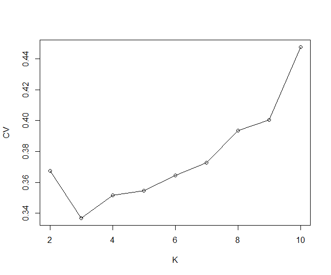
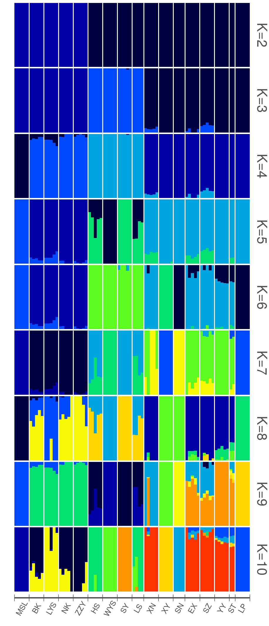
Based on the 13990 neutral SNPs (removing outlier loci identified by Arlequin and BayeScan from 16592 SNPs) and using Admixture, we observed three separate ancestry groups: L. tulipifera in North America (NA), L. chinense in eastern China (CE) except for the XN population, and L. chinense in western China (CW) (Fig. 1A). The Admixture plots and cross-validation error of each K (K = 2 to 10) are shown in Additional file 2: Fig. S1 and Additional file 3: Fig. S2, respectively. For the PCA (principal component analysis), the first principal component (PC1) separated L. chinense from L. tulipifera (P = 1.68 E-15), while the second principal component (PC2) separated CE from CW except for the XN population (P = 4.27 E-36) (Fig. 1B). The neighbor-joining tree further revealed that 17 populations were divided into three clusters, NA, CE, and CW, except for the XN population of CE clustering into CW (Fig. 1C). NA was genetically closer to CW than to CE. The AMOVA results also showed that genetic variation mainly existed among groups (68.78%, FCT = 0.69, P < 0.00001; Table 1). The genetic diversity analysis results showed that the genetic diversity of L. tulipifera populations is higher than that of L. chinense populations as a whole (Table 2). The genetic differentiation statistics results showed a high degree of genetic differentiation between L. tulipifera and L. chinense (Fig. 1D) (Fst = 0.86111). In addition, obvious genetic divergence was observed between CE and CW (Fst = 0.16935). Furthermore, we found that the genetic differentiation between NA and CE was slightly higher (Fst = 0.76841) than that between NA and CW (Fst = 0.75842).
Table 1 Hierarchical AMOVAs for SNP variations surveyed in Liriodendron.
|
Source of variation
|
d.f.
|
Sum of squares
|
Variance components
|
Percentage of variation
|
Fixation indices
|
P-value
|
|
Among groups
|
2
|
142505.59
|
1356.35
|
68.78
|
FCT = 0.69
|
P < 0.00001
|
|
Among populations within groups
|
14
|
19645.82
|
94.26
|
4.78
|
FSC = 0.15
|
P < 0.00001
|
|
within populations
|
143
|
74569.45
|
521.46
|
26.44
|
FST = 0.74
|
P < 0.00001
|
d.f.: degree of freedom.
Table 2 Details of the population locations, sample sizes, genetic diversity, voucher numbers and depositary of 17 populations of Liriodendron.
|
Pop ID
|
locations
|
Lat
|
Lng
|
Alt
|
N
|
NA
|
PPA
|
HE
|
Voucher numbers & depositary
|
|
NA
|
United States
|
-
|
-
|
-
|
25
|
6535
|
39.4
|
0.084
|
-
|
|
MSL
|
Missouri
|
38.87
|
-92.23
|
245
|
5
|
2772
|
16.7
|
0.060
|
00081690, PE
|
|
BK
|
North Carolina
|
36.07
|
-77.15
|
8
|
5
|
3876
|
23.3
|
0.078
|
00318635, NAS
|
|
LYS
|
Louisiana
|
30.42
|
-91.02
|
18
|
5
|
3284
|
19.8
|
0.071
|
01899157, PE
|
|
NK
|
South Carolina
|
33.83
|
-80.82
|
65
|
5
|
3961
|
23.9
|
0.079
|
00318637, NAS
|
|
ZZY
|
Georgia
|
34.64
|
-84.76
|
230
|
5
|
3628
|
21.8
|
0.075
|
00318634, NAS
|
|
CHN
|
China
|
-
|
-
|
-
|
55
|
10477
|
63.1
|
0.073
|
-
|
|
CE
|
Eastern China
|
-
|
-
|
-
|
24
|
4324
|
26
|
0.058
|
-
|
|
HS
|
Huangshan, Anhui
|
30.17
|
116.1
|
1250
|
5
|
2329
|
14.0
|
0.050
|
00318611, NAS
|
|
WYS
|
Wuyishan, Jiangxi
|
27.92
|
117.8
|
1000
|
5
|
1474
|
8.9
|
0.036
|
00081629, PE
|
|
SY
|
Songyang, Zhejiang
|
28.50
|
119.6
|
138
|
5
|
2465
|
14.8
|
0.052
|
00081550, PE
|
|
LS
|
Lushan, Jiangxi
|
29.53
|
116
|
1167
|
4
|
2345
|
14.1
|
0.054
|
20010020006, NJFU
|
|
XN
|
Xianning, Hubei
|
29.8
|
114.2
|
68
|
5
|
3023
|
18.2
|
0.062
|
20010020089, NJFU
|
|
CW
|
Western China
|
-
|
-
|
-
|
31
|
8457
|
50.9
|
0.072
|
-
|
|
XY
|
Xuyong, Sichuan
|
28.2
|
105.5
|
800
|
5
|
2148
|
12.9
|
0.047
|
0028959, CDBI
|
|
SN
|
Suining, Hunan
|
26.33
|
110.2
|
1500
|
4
|
1904
|
11.5
|
0.049
|
00081582, PE
|
|
EX
|
Exi,
Hubei
|
30.3
|
109
|
1180
|
5
|
3448
|
20.2
|
0.064
|
00081593, PE
|
|
SZ
|
Sangzhi, Hunan
|
29.15
|
110.2
|
1200
|
5
|
3313
|
19.9
|
0.064
|
00318629, NAS
|
|
YY
|
Youyang,
Sichuan
|
28.82
|
108.8
|
890
|
5
|
2780
|
16.7
|
0.060
|
01859555, PE
|
|
ST
|
Songtao, Guizhou
|
26.8
|
109.5
|
1050
|
2
|
1683
|
10.1
|
0.055
|
00875730, PE
|
|
LP
|
Liping, Guizhou
|
26.34
|
109.19
|
421
|
5
|
2130
|
12.8
|
0.048
|
20010020014, NJFU
|
Pop ID: population code, Lat: latitude, Lng: longitude, Alt : altitude, N: number of individuals, NA: number of polymorphic alleles, PPA: percentage of polymorphic alleles, HE: Nei’s 1987 measure of nucleotide diversity, NA: L. tulipifera populations, CHN: L. chinense populations, CE: eastern populations of L. chinense, CW: western populations of L. chinense; PE: Herbarium code of Beijing Institute of Botany; NAS: Herbarium code of Jiangsu Institute of Botany; NJFU: Herbarium code of Nanjing Forestry University; CDBI: Herbarium code of Chengdu Institute of Biology.
Fig. 1. Population genetic structure of Liriodendron. (A) The Admixture plots (K = 2 and 3) based on 13990 neutral loci. (B) The PCA result based on 16592 SNPs identified from Liriodendron. The 17 colors correspond to 17 populations from 3 groups. (C) Neighbor-joining phylogenetic tree of Liriodendron based on 16592 SNPs, with the evolutionary distances measure by p-distances with phylip. The three colors correspond to the 3 groups. (D) Matrix of the pairwise Fst of 17 populations in Liriodendron.
To provide insight into the roles of environmental factors in population genetic structure and their contribution to this population structure, RDA was performed. The RDA results are shown in Table 3 and Fig. 2. First, the interactive-forward-selection analysis detected the top 16 most influential environmental variables from 55 environmental variables. The 16 environmental variables included two temperature variables (bio2 and bio7), three precipitation variables (bio13, bio15 and bio17), 6 solar radiation variables (srad1, srad2, srad5, srad6, srad7 and srad10) and 5 wind speed variables (wind2, wind7, wind8, wind9 and wind10). The RDA results showed that the correlation between 16592 alleles and 16 environmental variables was 1.000 on axes 1 and 2. The eigenvalue ratios of axes 1 and 2 were 32.10% and 8.38%, respectively. Sixteen environmental factors divided the 17 populations of Liriodendron into three groups. Axis 1 (RDA 1) separated L. chinense from L. tulipifera, while axis 2 (RDA 2) separated CE from CW except for the XN population (Fig. 2). Among the 16 environmental factors, 8 environmental factors had a significant influence on the population genetic structure of Liriodendron (Table 3). The eight environmental factors included one temperature variable (bio2), three precipitation variables (bio13, bio15 and bio17), three solar radiation variables (srad2, srad5 and srad6) and one wind speed variable (wind2). The results suggested that precipitation and light play key roles in shaping the population structure of Liriodendron.
Table 3 Effects of 16 environmental variables on and their explained contributions to the population genetic structure of Liriodendron.
|
variables
|
Explains%
|
pseudo-F
|
P-value
|
P-value correction
|
|
bio15
|
30.4
|
6.6
|
0.002
|
0.004
|
|
srad6
|
30.0
|
6.4
|
0.002
|
0.004
|
|
srad5
|
29.8
|
6.4
|
0.002
|
0.004
|
|
bio2
|
28.9
|
6.1
|
0.002
|
0.004
|
|
bio13
|
21.7
|
4.2
|
0.002
|
0.004
|
|
bio17
|
21.5
|
4.1
|
0.002
|
0.004
|
|
srad2
|
20.1
|
3.8
|
0.002
|
0.004
|
|
wind2
|
19.9
|
3.7
|
0.002
|
0.004
|
|
srad7
|
17.6
|
3.2
|
0.006
|
0.01067
|
|
bio7
|
15.2
|
2.7
|
0.008
|
0.0128
|
|
srad10
|
10.7
|
1.8
|
0.054
|
0.07733
|
|
wind10
|
10.1
|
1.7
|
0.066
|
0.08123
|
|
wind9
|
9.8
|
1.6
|
0.058
|
0.07733
|
|
srad1
|
7.4
|
1.2
|
0.208
|
0.23771
|
|
wind8
|
6.3
|
1.0
|
0.402
|
0.402
|
|
wind7
|
6.0
|
1.0
|
0.396
|
0.402
|
Explains%: The contributions of variables to the population genetic structure.
Fig. 2. Redundancy analysis of Liriodendron showing the relative contributions of 16 environmental variables to the population genetic structure. The biplot depicts the eigenvalues and the lengths of eigenvectors for the RDA, and the color gradient corresponds to genetic diversity.
Ecological niche differentiation analysis
The SEEVA results showed that 22 ecological factors undergo significant divergence (D > 0.75, P < 0.0016) between L. chinense and L. tulipifera habitats (Fig. 3; Additional file 4: Table S2). In addition, 6 ecological factors have diverged significantly (D > 0.75, P < 0.0016) in the eastern and western habitats of L. chinense (Fig. 3; Additional file 4: Table S2).
Fig. 3. The divergence index and impact index shown as bar diagrams for elevation and 55 climatic variables between sister species and sister groups. (A) The divergence index and impact index shown as bar diagrams for elevation and 55 climatic variables between L. chinense and L. tulipifera. (B) The divergence index and impact index shown as bar diagrams for elevation and 55 climatic variables between east and west groups.
Leaf shape analysis
The results of leaf shape analysis showed that the leaf shape variation was the most abundant in CW, and the variation range covered almost all the leaf variation in CE and NA (Fig. 4). However, CE and NA have common leaf variations and unique leaf variations. Furthermore, the statistical results of the number of cracks in leaves showed that the number for L. chinense ranged from 3 to 6, and 92.14% of the leaves had 3 cracks. However, the number of cracks in the leaves of L. tulipifera ranged from 3 to 9, among which 5 and 3 were common, accounting for 63.10% and 16.67%, respectively (Additional file 5: Table S3).
Fig. 4. Leaf shape variation distributions in three groups of Liriodendron (X-axis: The ratio of x1 and x2; Y-axis: The ratio of y1 and y2; x1: The vertical distance from the right lateral sinus to the primary vein. x2: The vertical distance from the right lateral lobe to the primary vein. y1: The vertical distance from the right lateral sinus to the leaf base. y2: The vertical distance from the right apical lobe to the leaf base) (Confidence interval: 95%).
Characterization of environment-associated loci
There were 1917 and 1808 outlier sites identified by Arlequin and BayeScan, respectively (Additional file 6: Table S4 and Additional file 7: Table S5). In total, 1123 outlier loci were identified by both Arlequin and BayeScan. The results of the environment-associated analysis showed that 858 EAL associated with at least one environmental factor were identified by LFMM (Additional file 8: Table S6). Furthermore, LFMM analysis showed that precipitation seasonality (bio15), elevation, precipitation in the driest quarter (bio17), precipitation in the warmest quarter (bio18), the mean diurnal range of temperature (bio2), solar radiation in May (Srad5) and water vapor pressure in July (vapr7) were associated with the highest numbers (> 70) of EAL (Additional file 8: Table S6).
GO and KEGG enrichment analysis
The genomic contexts of the 858 EAL were determined based on the L. chinense reference genome [52]. We found that 667 EAL were associated with 464 genes, and 191 EAL corresponded with the intergenomic regions (Additional file 8: Table S6). The results of GO annotation showed that these genes represented a broad range of biological processes, molecular functions and cellular components (Additional file 9: Fig. S3). Furthermore, some genes are considered to be involved in the response to biotic and abiotic stresses, phenology, disease resistance and hormonal responses (Additional file 10: Table S7), such as ARF1 (ethylene and cytokinin responses) [53], RAP2-7 (ethylene-responsive transcription factor), RP/EB family member 1B-like (response to wounding) [54], FRIGIDA-like (flowering time) [55], UVR8 (photomorphogenesis and stress acclimation) [56] and RGA2-like (disease resistance protein) [57], were identified in other plants. In addition, we found some genes involved in the response to biotic and abiotic stresses, stimuli, immune responses, growth and development, and programmed cell death by Gene Ontology annotation (Additional file 11: Table S8).
The enriched GO terms biological process, cellular component and molecular function are shown in Additional file 9: Fig. S3. Genes of GO terms such as ‘inorganic diphosphatase activity’, ‘protein transport’, ‘deoxyribonucleotide metabolic process’, ‘protein secretion’, and ‘ubiquitin-like protein-specific protease activity’ were highly enriched. Pathway enrichment analysis revealed that genes involved in plant-pathogen interactions, phosphatidylinositol signaling systems, ubiquitin-mediated proteolysis, carotenoid biosynthesis, alpha-linolenic acid metabolism and phagosomes were significantly enriched (Fig. 5). Related studies have shown that these biological pathways play vital roles in plant growth, development, stress, immune response and photosynthesis.
Fig. 5. The plots of the KEGG enrichment analysis results.