The hydrological, geological and meteorological conditions in southwestern China are relatively complex, so that the land surface deformation presents various features. Aiming at 58 Crustal Movement Observation Network of China (CMONOC) stations across four provinces in Southwestern China, we adopt an improved clustering algorithm to classify 49 stations into 12 clusters with different similarity levels. Our results show that the average annual signals of GPS stations within each cluster have strong consistency, while obvious differences exist among the 12 clusters, indicating that clustering algorithm helps to describe surface deformation features more accurately in regions with complex conditions. We then combine other earth observation techniques, such as the Gravity Recovery and Climate Experiment (GRACE) satellite datasets and surface loading models (SLM), and observe that GPS, GRACE and SLM have strong correlation in their monthly displacement series at GPS stations. After excluding non-clustered stations according to our previous clustering results, the correlation coefficients of GPS/GRACE and GPS/SLM are enhanced. Also, the RMS reduction rates of GPS coordinate time series have been improved after deducting displacements obtained from GRACE and SLM, thus the clustering algorithm proves to be effective in improving the consistency of three techniques in joint detection of surface deformation. Moreover, the vertical displacements of four riverside GPS stations in the Three Gorges Reservoir (TGR) area show significant negative correlation with water level of TGR, hence we conclude that the Three Gorges Dam (TGD) may directly affect the consistency of GPS annual signals of its upstream and downstream GPS stations.
Full paper
Application of an Improved Clustering Approach on GPS Height Time Series at CMONOC Stations in Southwestern China
https://doi.org/10.21203/rs.3.rs-763039/v1
This work is licensed under a CC BY 4.0 License
Journal Publication
published 01 Dec, 2021
You are reading this latest preprint version
clustering algorithm
CMONOC stations
GPS height time series
land surface deformation
GRACE
SLM
In the past 20 years, many researchers have used Global Positioning System (GPS) coordinate time series to carry out research in earth science from different aspects (Blewitt et al., 2001; Dong et al, 2002; Williams et al., 2004; Ray et al., 2008; Langbein, 2008; van Dam et al., 2010; Jiang et al., 2013; Gu et al., 2017). In addition to GPS technology, comprehensive usage of other earth observation methods, such as the Gravity Recovery and Climate Experiment (GRACE) satellite datasets, surface loading models (SLM), etc., help to crosscheck the effectiveness of these techniques. Thus, advantages of different techniques in the application of earth science can be combined, which would be more reliable and accurate in reflecting the real surface movement characteristics (Tesmer et al., 2011). However, there are inevitably some abnormal signals caused by local geophysical factors in GPS coordinate time series observed by GPS, which is unfavorable for the consistency among GPS, GRACE and SLM.
In order to identify local GPS stations that are affected by abnormal geophysical signal interference or GPS technical errors, Tesmer et al. (2009) proposed a station clustering algorithm. This approach was to find local stations with similar annual variations among dense GPS stations, then to group them into a cluster according to two criteria, so as to effectively eliminate regional abnormal stations and extract the common annual variation features. Subsequently, Wu et al. (2021) proposed an improved clustering algorithm through adding annual phase of GPS stations as the third criterion. They found that the clustering accuracy under constraint of annual phase was improved, and the annual signals of GPS stations within clusters had stronger consistency. This method helps to describe the surface deformation characteristics more accurately inside a region.
Freymueller (2009) analyzed seasonal variations at GPS stations located in northern North America and the Arctic. He found that the seasonal variations at most GPS stations were not manifested as annual sinusoidal signals, but annual recurring signals. In China, however, many GPS stations show obvious annual sinusoidal signals, especially in the southwestern region (Zhao, 2017; Zhan et al., 2017). Therefore, when estimating annual signals of GPS height time series, the accuracy of annual amplitude and phase can be higher, thus the constraint effect of annual phase can be better in the improved clustering method proposed by Wu et al. (2021).
In this study, the improved clustering algorithm is applied to 58 CMONOC stations in Southwestern China. The three clustering criteria are interstation distances, WRMS differences and annual phase differences among GPS stations. Firstly, threshold values of the three criteria were selected and evaluated simultaneously to keep the best agreement of internal signals, so that a larger number of clusters and GPS stations in a local area can be obtained. Then improved clustering algorithm is executed based on the obtained optimal thresholds to obtain clustering results in Southwest China. Next, other earth observation techniques, including GRACE and SLM are employed to jointly detect the surface vertical deformation in this study area, to evaluate the consistency among these three techniques and effectiveness of the above clustering approach. Finally, the reason of several GPS stations that are not being grouped into clusters is discussed, and a special cluster located in the Sichuan Basin is deeply investigated, so as to determine potential reasons for the annual variations of its internal GPS stations.
1.1 GPS height time series
The GPS height time series analyzed in this study is provided by China Earthquake Administration (CEA) (ftp://ftp.cgps.ac.cn/), including both raw and detrended time series for all 260 CMONOC stations. CEA adopts GAMIT/GLOBK10.4 software (Herring et al., 2010) to process the GPS observations of CMONOC stations. After obtaining loosely constrained daily solutions, the daily solutions are transformed into International Terrestrial Reference Frame 2008 (ITRF08, Rebischung et al., 2012) by implementing a 7-parameter transformation through GLOBK processing. Details of GPS modeling and additional information can be found in the data processing manual (ftp://ftp.cgps.ac.cn/doc/processing_manual.pdf).
Spatial distribution of the selected 58 CMONOC stations in four southwestern provinces is shown in Fig. 1, and the GPS height time series span from 1999 to 2019. These stations can be divided into two types according to their construction time. Four stations, KMIN and KUNM in Kunming city, LUZH (Luzhou City, Sichuan) and XIAG (Dali, Yunnan) belong to the first stage of CMONOC project (CMONOC-I), with effective time spans of more than 10 years (14 years for KUNM, and 20 years for the other three stations). The remaining 54 stations were built during the second stage of CMONOC project (CMONOC-II) with effective time spans of 8–9 years. GPS stations in this region are densely distributed, since the selected area is located on southeastern edge of the Qinghai-Tibet Plateau, which is sensitive with crustal movement and hydrological climatic changes. By processing and analyzing accumulated long-term GPS observations, it is helpful to reveal the characteristics of crustal movement and water vapor changes in this region (Tang et al., 2013; Jiang et al., 2017). After checking outliers and offsets in raw series, the detrended series were acquired through linear fitting. To avoid some unrecognizable and unknown offsets, we use the raw GPS height time series for clustering analysis, thus it is necessary to do some data preprocessing, including detection of outliers, offsets and abnormal nonlinear deformations.
1.2 Improved clustering algorithm
To effectively distinguish GPS height time series that are negatively affected by some local geophysical anomalies or technical defects, we apply the improved clustering algorithm to 58 CMONOC stations in Southwest China (Wu et al., 2021). Detailed procedures are as follows:
- Compute average annual series for each of the 58 CMONOC stations by stacking and averaging multi-years’ series into one year.
- Compute WRMS values of the one-year series for each station, and then form a WRMS difference matrix among stations (58×58, a symmetric matrix with diagonal elements as 0). Similarly, compute an interstation distance matrix among all stations with the same dimension. WRMS is calculated as follows:

where s(i) and g(i) represent the vertical displacement of GPS stations and its formal error or uncertainty at epoch i; n indicates the number of observations. In this case, n = 365. WRMS value reflects the strength of signal fluctuation at GPS stations. The larger WRMS values, the more obvious nonlinear variations in GPS stations.
- Estimate parameters of the annual amplitude and phase of GPS stations, as well as the annual phase differences among stations to obtain a phase difference matrix. These three matrices with the same dimensions are called as criteria matrices.
- Determine the thresholds of different similarity levels according to numerical values of the three criteria matrices, and then execute the clustering algorithm to detect spatially correlated clusters by step 1) searching similar stations with WRMS difference smaller than limit X, and interstation distance shorter than limit Y, as well as annual phase difference less than limit Z; step 2) classifying these groups of stations (no less than three) as clusters; step 3) eliminating overlapping stations among clusters by assigning them into biggest cluster to ensure that each station belongs to only one cluster.
- Iterate the above step for several times, each time with larger thresholds of X, Y and Z until most stations are grouped into one cluster. During iteration, stations grouped into clusters of the former iteration have to be removed.
In the above clustering process, the three criteria matrices are jointly used to determine several spatially correlated GPS stations in a cluster. These stations are close in distance with similar variations of annual amplitude and phase. For numerical values of the three matrices, we initially arrange four sets of thresholds, namely 0.5/150/10, 1.0/300/20, 1.5/450/30 and 2.0/600/40. For example, with respect to a cluster of level-one similarity, its internal GPS stations need to meet the WRMS difference of less than 0.5 mm, the interstation distance and the annual phase difference should be less than 150 km and 10 days, respectively.
To evaluate the degree of agreement between GPS stations within a cluster, we used an indicator, the maximal differential WRMS. That is, for a cluster containing three stations A, B and C, we firstly obtain the annual series difference among these stations, namely s(A)-s(B), s(A)-s(C) and S(B)-s(C), and then calculate WRMS values of the difference series, among which the maximum value is used as the index to measure consistency of GPS stations within this cluster. Different from Tesmer et al. (2009), the number of GPS stations contained in a cluster of Wu et al. (2021) is at least three, instead of two, so as to ensure that the GPS stations in each cluster can more robustly reflect the characteristics of regional surface deformation. In addition, our used thresholds are also different, which are determined by factors such as region scale, density of GPS stations and characteristics of annual signals.
2.1 Selection and evaluation of thresholds
Table 1 lists the clustering results based on our initially-set thresholds. After four-iterations, a total of 42 GPS stations are included in 10 clusters, while the remaining 16 stations are considered to be different with neighboring stations, thus they are not included in any cluster. Specifically, in the first iteration, the thresholds of three criteria matrices were set as 0.5 mm, 150 km and 10 days. In this case, only one cluster of level-one similarity is obtained, including three GPS stations. The maximal differential WRMS of this cluster is 2.02 mm. These three stations acquired from the first iteration were then removed and the thresholds were enlarged to perform the second iteration. At this stage, four clusters of level-two similarity are obtained, containing 18 GPS stations. In the third and fourth iterations, three and two clusters are obtained, respectively. With increasing thresholds, the maximal differential WRMS also increased, and the annual signal consistency of GPS stations within a cluster decreased correspondingly.
Table 1. Clustering results derived from initially-set thresholds
|
Similarity Level |
Thresholds (mm/km/day) |
No. of Stations |
No. of Clusters |
Maximal Differential WRMS (mm) |
|
1 |
0.5/150/10 |
3 |
1 |
2.02 |
|
2 |
1.0/300/20 |
18 |
4 |
2.82 |
|
3 |
1.5/450/30 |
15 |
3 |
2.97 |
|
4 |
2.0/600/40 |
6 |
2 |
2.93 |
|
Sum |
42 |
10 |
2.79 |
The selection of thresholds would affect the number of clusters at all levels of similarity and also the number of GPS stations. Therefore, the reason of those 16 stations that were not being classified into clusters probably may be due to too much strict thresholds of one criterion or more. To verify whether the initially-set thresholds are reasonable, the step lengths of these three criteria thresholds were increased, respectively, and the corresponding clustering results are listed in Table 2.
Table 2. Clustering results derived from several groups of thresholds
|
Thresholds Step Length |
Similarity Level |
Thresholds (mm/km/day) |
No. of Stations |
No. of Clusters |
Maximal Differential WRMS (mm) |
|
Group One (WRMS: +0.5 mm) |
1 |
1.0/150/10 |
3 |
1 |
2.02 |
|
2 |
2.0/300/20 |
20 |
4 |
3.26 |
|
|
3 |
3.0/450/30 |
20 |
4 |
3.41 |
|
|
4 |
4.0/600/40 |
3 |
1 |
2.33 |
|
|
Sum |
46 |
10 |
3.10 |
||
|
Group Two (Distance: +50 km) |
1 |
0.5/200/10 |
7 |
2 |
2.67 |
|
2 |
1.0/400/20 |
19 |
4 |
2.85 |
|
|
3 |
1.5/600/30 |
12 |
2 |
3.07 |
|
|
4 |
2.0/800/40 |
8 |
2 |
3.01 |
|
|
Sum |
46 |
10 |
2.89 |
||
|
Group Three (Phase: +5 days) |
1 |
0.5/150/15 |
3 |
1 |
2.02 |
|
2 |
1.0/300/30 |
23 |
5 |
2.96 |
|
|
3 |
1.5/450/45 |
16 |
4 |
2.66 |
|
|
4 |
2.0/600/60 |
7 |
2 |
3.11 |
|
|
Sum |
49 |
12 |
2.81 |
From group one and two in Table 2, when step length of WRMS increased by 0.5 mm and interstation distance increased by 50 km, the total number of clusters remained the same, while the number of clustered GPS stations increased by four compared with results in Table 1. Meanwhile, the maximal WRMS increased from 2.73 mm to 3.10 and 2.89 mm, respectively. For group three, if step length of annual phase difference increased by 5 days, the total number of clusters and the contained GPS stations obviously increased, with only slight change in the maximal differential WRMS, indicating that the initially-set thresholds of annual phase difference can be strict, and the results of group three in Table 2 can be appropriate. It not only guarantees a sufficient number of clusters and clustered GPS stations, but also keeps the clustering accuracy steady compared with clustering results in Table 1. Hence, we take group three as the final clustering results for later analysis.
2.2 Clustering results
Fig. 2 shows the average annual signals of GPS stations in 12 clusters from group three, namely C1-C12. In general, the annual signals in each cluster have high consistency, and most GPS stations in Southwest China have obvious annual sinusoidal signals, which further demonstrates that application of the third criterion matrix, that is, the annual phase difference, helps to identify GPS stations with similar motion features. Moreover, higher-level clusters contain more GPS stations with obvious sinusoidal signals, while lower-level clusters contain less.
Specifically, C1 is the only level-one similarity cluster, with the highest similarity level and the strongest consistency of annual signal among internal GPS stations. C2-C6 are five level-two clusters, with a lower similarity level than C1, but also show strong consistency among annual signals of their own internal stations. C7-C10 represent four level-three clusters, and the annual signals of internal stations tend to be consistent overall, although there are a few stations show inconsistency at some certain period of a year. C11 and C12 indicate two level-four clusters, with the lowest similarity level, and the annual signal consistency of their internal stations is the weakest among all 12 clusters.
Fig. 3 depicts the geographic distribution of 12 clusters. In general, clusters with high-level similarity are concentrated in the middle of the region, while those with low-level similarity are mostly distributed in the edge. Combined with Fig. 2, it can be found that most GPS stations located in southern Sichuan and Yunnan Province show obvious annual sinusoidal signals, while cluster C8 in the Sichuan Basin and C4 in the Western Sichuan Plateau do not.
After four-iteration process, 12 clusters are generated containing 49 GPS stations, while the remaining 9 stations represented as black dots in Fig. 3 are preliminarily considered as stations with local abnormal signals. These stations are mainly distributed at the marginal area. Generally, the number of adjacent stations of a marginal station is less than that of an internal station, so there is less opportunity for the marginal station to form a cluster with at least two similar surrounding stations. This is probably the reason why stations assumed as with abnormal signals are more distributed in the marginal area.
Fig. 3 also shows that the distribution patterns of all 12 clusters are different. Some clusters show an approximate linear shape, such as C1, C3 and C10, while some present a nest-like distribution, like C2, C5 and C7. These different distribution patterns are partly due to the insufficient density of GPS stations, because there are more clusters showing as nest-like shape when involved stations are dense enough. However, based on the current density of GPS stations in this region, surface deformation characteristics can also be displayed in Fig. 3 to some extent.
2.3 Annual signal analysis at GPS stations
Based on the above clustering results, we further analyze the annual motion characteristics of the GPS stations in Southwest China, as shown in Fig. 4. Among the four southwestern provinces, the annual amplitudes of three GPS stations in Guizhou Province are the smallest, while those in the remaining three provinces have much larger annual amplitudes, with average annual amplitudes of GPS stations in Sichuan, Yunnan and Chongqing as 4.6, 6.2 and 5.4 mm, respectively. Stations with the largest annual amplitudes are mainly concentrated in central and western Yunnan, which is consistent with existing research results (Sheng et al., 2014; Jiang et al., 2017).
For the annual phase, the study area has shown obvious systematic changes. From western Yunnan along the Hengduan Mountains to the north of Western Sichuan Plateau, the annual phase of GPS stations gradually decrease from April to February. However, those of GPS stations in eastern Sichuan, namely the Sichuan Basin and Chongqing, are increased from May to July. Interestingly, for several GPS stations along the Yangtze River, starting from eastern station CQWZ in Chongqing, passing upstream through stations CQCS, LUZH, and SCJU, the annual phases gradually decrease from July to April. We suppose the potential reason may be the diverse hydrological conditions along the Yangtze River.
In addition, we observe that for clusters of high similarity levels (such as C1 to C6), their internal GPS stations have similar annual amplitudes and phases, while for clusters with lower similarity levels (such as C7 and C12), the annual phase of internal stations can be within thresholds of the corresponding level, but their annual amplitudes are quite different. The remaining 9 stations are mainly distributed at the edge of the area. Some stations have obvious abnormal annual phases, such as SCGY, SCMX and YNGM marked in Fig. 4. Such stations will be mainly analyzed in section 3.1.
To fully and truly detect the characteristics of land surface deformation, it is necessary to integrate other geodetic techniques, such as GRACE and SLM. The employed GRACE Level-2 GSM data were the latest RL06 version released by the Center for Space Research (CSR) at the University of Texas (Bettadpur, 2007; Gao et al., 2019). The time span was 163 months from April 2002 to June 2017, after excluding missing months. Compared with the last version RL05, RL06 data adopts some new background gravity field models and improved processing methods. The north-south stripes have been significantly reduced compared with RL05 data (Save et al., 2016; Save, 2019), among which quadratic polynomial fitting method (Swenson and Wahr, 2006) and the Gaussian filtering with a radius of 300 km were used to reduce stripe errors. Since the original C20 terms of the SH coefficients have large uncertainty, it needs to be replaced by estimates from satellite laser ranging (SLR, Cheng et al., 2013). In addition, replacement of the first-degree SH coefficients is also necessary, and we used the replacement values provided by Swenson et al. (2008). In order to weaken the influence of high-frequency errors, all SH coefficients were truncated to the 60th order/degree. In this study, we apply the software GRAMAT developed by Feng (2019).
Several organizations around the world, such as NASA, GFZ and EOST, have established different SLM models based on geophysical observation data and Earth models, and have provided a variety of land surface loading products (Li et al., 2020). In this study, the loading grid product provided by GFZ (Dill and Dobslaw, 2013) was used to calculate the displacement series generated by non-tidal atmospheric and oceanic loading, as well as hydrological loading at CMONOC stations (Yuan et al., 2018; Wu et al., 2019). Considering that the temporal resolution of GRACE data is one month, the single-day series of GPS and SLM were also averaged to obtain monthly displacement series. Correlation coefficients and RMS reduction rates among the three types of monthly displacement series, including GPS, GRACE and SLM, are shown in Fig. 5 and Fig. 6.
As shown from Fig. 5, the surface displacement series obtained by three types of techniques have strong correlations, with average correlation coefficients as 0.62, 0.70 and 0.87 for GPS/GRACE, GPS/SLM and GRACE/SLM, respectively, at 58 GPS stations. In comparison, the correlation coefficients for GPS/GRACE and GPS/SLM are lower than that for GRACE/SLM. This is because GPS is more sensitive to surface deformation caused by local loading effects, and could continuously monitor millimeter-level changes at GPS stations. Specifically, GPS belongs to a kind of point measurement mode (Nahmani et al., 2012; Wei et al., 2015). However, GRACE uses a surface measurement mode with spatial scale of ~400 km, while the spatial resolution of SLM provided by GFZ is also close to that of GRACE. Such local changes will not be recognized by GRACE and SLM as effectively as GPS (Wang et al., 2014), thus causing the sensitivity difference of these techniques in detecting land surface displacement.
From Fig. 6, we observe that for all 58 GPS stations, after deducting GRACE and SLM series from GPS series, the RMS of GPS time series decrease at 51 and 50 stations, respectively, with average RMS reduction rates of 20.0% and 21.8%. Stations with better GRACE correction effect are distributed in western part of the region, while the distribution of seven stations with poor correction effect is dispersive (Fig. 6a). From Fig. 6b, stations with better SLM correction effect are distributed in the Hengduan Mountains, while those in the Sichuan Basin and some along the Yangtze River display poor correction effect. Comparing Fig. 6a with 6b, the RMS reduction rates of four common stations GZFG, SCJU, SCMX and YNGM are negative, while these stations all show positive values in Fig. 6c. Therefore, it is reasonable to believe that the GPS monthly series of these four stations probably contain some abnormal local signals, which could be detected by joint employment of GPS, GRACE and SLM.
To illustrate the ability of our improved clustering algorithm to detect regional anomaly signals at GPS stations, Table 3 lists the average values of correlation coefficients and RMS reduction rates at all 58 stations, 49 stations of the clustering results (C1-C12), and 26 stations of high similarity level clusters (C1-C6). Before executing clustering algorithm, the average correlation coefficients of GPS/GRACE and GPS/SLM at all 58 stations are 0.62 and 0.70, respectively. After clustering process, the corresponding values for 49 stations in 12 clusters increase to 0.65 and 0.73. In particular, for 6 clusters of similarity level one and two (26 stations in total), the corresponding values increase to 0.67 and 0.77. Similarly, before clustering, the average RMS reduction rates of GPS-GRACE and GPS-SLM series at all 58 stations are 20.0% and 21.8%, respectively. After clustering, the corresponding values for 49 stations in 12 clusters increase to 23.0% and 24.2%, while for 26 stations in cluster C1-C6, the values increased to 26.6% and 33.0%, respectively.
Table 3. Average correlation coefficients and RMS reduction rates at all 58 stations, 49 stations of all 12 clusters, and 26 stations of 6 clusters (C1-C6).
|
Stations |
Correlation Coefficient |
RMS reduction rate (%) |
||||
|
GPS/ GRACE |
GPS/ SLM |
GRACE/ SLM |
GPS-GRACE |
GPS-SLM |
GRACE-SLM |
|
|
All 58 |
0.62 |
0.70 |
0.87 |
20.0 |
21.8 |
35.6 |
|
49 in C1-C12 |
0.65 |
0.73 |
0.86 |
23.0 |
24.2 |
34.5 |
|
26 in C1-C6 |
0.67 |
0.77 |
0.86 |
26.6 |
33.0 |
36.1 |
3.1 Analysis of GPS stations with local abnormal signals
In Sect. 2.2, the remaining 9 stations are not included in their surrounding clusters, and most of them are located at edge of the area. Preliminary analysis suggests that this is because the number of neighboring stations is comparatively small for marginal stations, and they need at least two similar stations to form a cluster, so that the opportunity of being isolated is larger for these marginal stations compared with central stations. These stations are not always the stations containing abnormal signals that need to eliminate, since regional station with abnormal signal means that the attribute of the station itself is different from surrounding stations. For example, the annual phases of three stations, namely SCGY, SCMX and YNGM, are obviously different from those of the surrounding stations (Sect. 2.3). Figure 7 shows the annual signals of these three stations and their neighboring stations. It can be observed that obvious differences exist from panel a, b and c.
In addition to annual phase, WRMS of GPS annual signal is another factor that could affect the clustering results. When the annual amplitude of a station is large, the WRMS value of its annual signal is also large. During clustering process, this kind of station will be eliminated because its WRMS difference with surrounding stations would exceed the corresponding threshold. Taking station CQWZ as an example, its WRMS is 4.4 mm, while the average WRMS of its neighboring cluster C8 is 2.5 mm (Fig. 7d). The resulted WRMS difference exceeds the threshold of level-three similarity, thus our final clustering result does not contain CQWZ in C8.
Another three stations YNJP, YNMZ and YNWS located in southeast of the study area are also not included in any cluster, with clusters C3 and C10 distributed around them. Cluster C3 belongs to level-two similarity cluster, with differences of WRMS and annual phase among its internal stations less than 1.0 mm and 30 days, respectively. The annual phase difference between these three stations and station YNXP in C3 is greater than 30 days, so they are not included in C3. Similarly, the WRMS difference between these three stations and station KUNM in C10 is larger than 1.5 mm, thus they are not included in C10 either. Note that Tesmer et al. (2009) set at least two stations in a cluster. However, the above-improved clustering algorithm employed a more stringent standard. That is, a cluster must have at least three stations. If the minimum number of stations within a cluster is reassigned to two, two stations YNJP and YNWS can also form a new cluster.
3.2 Cluster C8 and the Three Gorge Reservoir area
As mentioned in Sect. 2.2, GPS stations in cluster C8 exhibit non-sinusoidal signals, but annual recurring signals. C8 is located in eastern part of Sichuan Basin, among which station CQCS is situated in Changshou District, Chongqing, adjacent to the riverbank of Yangtze River. The annual signals of four GPS stations contained in C8 show strong consistency, gradually increase from January, reaching maximal positions in July, and then decrease to arrive at the toughs in November, then gradually increase by the year end. As displayed in Fig. 7d, CQWZ is not grouped into cluster C8 due to its large WRMS value. Located in Wanzhou District, Chongqing, also a riverside station, this station shows similar annual variation trend with respect to station CQCS.
Yuan et al. (2018) analyzed the impact of environmental loadings on CMONOC stations and found that the root mean square (RMS) of most stations decreased after environmental loading corrections (ELCs). Nevertheless, the RMS value of station CQCS increased significantly after ELCs. Their analysis believed this may because the hydrological model adopted by GFZ products could not faithfully reflect hydrological changes in the Three Gorges Reservoir (TGR) area, thus resulting in inaccurate hydrological loading series at CQCS. The abnormality of CQCS can also be found in our experiment, as shown in Fig. 6b.
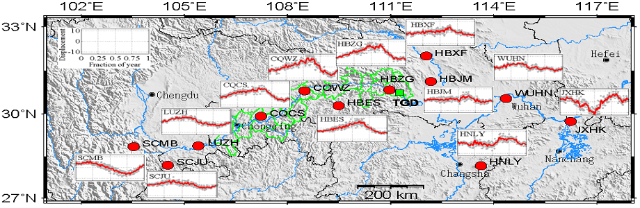
To verify whether these special signals of GPS vertical displacement in cluster C8 are related to the TGR area, we analyze 12 riverside CMONOC stations. The spatial distribution and average GPS annual signals of these 12 stations are shown in Fig. 8. Divided by TGD, there are 7 stations upstream and 5 stations downstream. Except for two stations, namely LUZH and WUHN, the remaining 10 stations belong to CMONOC-II with starting epoch at around March 2010.
From Fig. 8, we can see that there are four CMONOC stations within the TGR area, namely HBZG, HBES, CQWZ and CQCS. The GPS annual variations of these four stations are roughly the same, gradually rising from beginning of the year, reaching to peaks in July and then dropping to minimum values from November to December, finally rising again by the year end, with a range of 15–20 mm throughout the whole year. However, for three stations WUHN, JXHK and HNLY, located downstream of the TGD, together with two stations HBXF, HBJM along riverside of the Hanjiang River, the average GPS annual signals do not have a consistent variation trend. Among them, the maximum values of HBXF and HBJM also occur in July. These two stations also have a similar upward and downward trend like the above four upstream stations in the TGR area, but the variations are comparatively small, only less than 10 mm throughout a year. Another interesting phenomenon is that HBZG is about 400 km away from CQCS and only 120 km away from HBJM. However, the GPS annual signal of HBZG is quite similar to CQCS, but different from HBJM. Therefore, we think that TGR probably has a significant impact on the annual signal consistency among GPS stations upstream and downstream the TGD.
TGR is a long narrow river-shaped reservoir, extending from Chongqing in the west to Yichang in the east, with a length of more than 600 km. This area is mountainous and steep, filled with numerous valleys and waterways, thus it is prone to geological disasters, such as landslides and debris flows. TGR was first impounded to 175 m in 2008. Its water level then keeps changing annually between 145 and 175 m, and previous researches have already proved that the periodic rise and fall of TGR water level had an important impact on local geology and ecological environment (Liao et al., 2012; Jian et al., 2014). Figure 9 shows daily time series of the TGR water level change from 2010.0 to 2020.0. This dataset is acquired from website of the China Three Gorges Corporation (https://www.ctg.com.cn/sxjt/sqqk/index.html). To further compare the average annual signals of four GPS stations in the TGR area, the average annual water level of TGR within 10 years is also calculated. Among these four GPS stations, HBZG is closest to the TGD, only about 20 km, hence it is selected to analyze the relationship between TGR water level and GPS vertical displacement, as shown in Fig. 10.
It can be seen from Fig. 10 that there is an obvious negative correlation between GPS vertical displacement at station HBZG and the TGR water level, with correlation coefficient as -0.93. Specifically, in the first half year, the displacement rises gradually with declining TGR water level, which falls to the lowest value of 145.4 m on DOY 171 (20th June). At this moment, the displacement of HBZG almost reaches its first peak in a year. With annual arrival of flood season, upper reaches of the Yangtze River experiences an increasing rainfall, thus the TGR water level gradually rises to reach a small peak of 152.9 m during flood season on DOY 207, that is 26th July. At this time, the position of HBZG also drops to its bottom during the flood season. Afterwards, the TGR water level declines again and reaches its second trough of the whole year, with 147.8 m on DOY 230, namely 18th August. Correspondingly, the displacement also reaches the annual maximum value two days later. Then, TGR starts the main impoundment period of a year, reaching the annual peak water level of 174.6 m on DOY 304 (31st October). In the last two months of the year, the TGR water level is basically stable with only a slight decrease, while the position of HBZG gradually decreases to the annual minimum, and then also remains stable in November and December.
In recent years, many scholars have used other earth observation methods, such as Interferometric Synthetic Aperture Radar (InSAR), to conduct studies on land surface deformation in the TGR area, including landslides of Huangtupo and Zhaoshuling (Liu et al., 2013; Shi et al., 2016), Fanjiaping (Fan et al., 2017) and Shuping (Liao et al., 2012). They found that the topography of valley slope, local rainfall and water level changes in the reservoir area were important factors leading to landslides. CMONOC stations are mostly built on bedrock or stable soil, thus rainfall has a weak influence on the position change of GPS stations. Therefore, the rise and fall of TGR water level has become an important factor that affects the station displacement. When TGR water level drops in the first half year, the downward force caused by reservoir water gravity on the surrounding rock masses becomes smaller, so that the stations’ position gradually rebound. On the contrary, during the impoundment period from August to October, the water level gradually rises, which increases the downward pressure from reservoir water, hence stations’ displacement gradually decrease.
Corresponding to the double troughs in annual signal of TGR water level, GPS vertical annual displacement at HBZG also shows significant double peaks during the same period. However, for the other three GPS stations in TGR area, the displayed double-peaks are not obvious. This is probably because the closer to TGD, the deeper of the reservoir water, thus its pressure change on surrounding rock masses would be larger, and ability of GPS stations to perceive pressure changes would also be stronger.
In this paper, an annual phase augmented clustering algorithm was applied to 58 CMONOC stations located in Southwest China. By setting the threshold values of three clustering criteria, 49 GPS stations were classified into 12 clusters of different similarity levels. We find that GPS stations in Southwest China show obvious annual recurring signals, and most of them have sinusoidal shapes. The improved clustering method can effectively extract GPS stations with similar annual signals into clusters. The higher similarity level of a cluster, the higher consistency of the average annual signal for its internal GPS stations, and the stronger ability to reflect overall characteristics of the regional surface deformation.
We then combined other techniques, such as GRACE and SLM, to analyze the characteristics of land surface deformation in the study region. Our results show that GPS, GRACE and SLM monthly time series have strong correlation at GPS stations in Southwest China. After excluding stations with abnormal signals based on the clustering results, the correlations among GPS, GRACE and SLM monthly series are enhanced. At the same time, when using GRACE and SLM series to correct GPS series, RMS reduction rate of the GPS coordinate time series is also improved after excluding stations with abnormal signals. Therefore, we conclude that the improved clustering algorithm is effective for improving the consistency of these three techniques in joint detection of land surface deformation.
Finally, we find that the average annual signals of four riverside GPS stations in the TGR area show a consistent variation trend. Their GPS vertical displacements are obviously negatively correlated with TGR water level, with correlation coefficient of -0.93 for station HBZG. Upstream and downstream the TGR, there are no apparent correlation between GPS annual signals and the TGR water level, thus we conclude that TGD probably has affected the consistency of annual signals at GPS stations upstream and downstream TGD.
Availability of data and materials: GPS datasets employed in this manuscript was acquired from the China Earthquake Administration (ftp://ftp.cgps.ac.cn/products/position/gamit/). If this site is not working, data will be available from the correspondence author on reasonable request.
Competing interests: The authors declare no conflict of interest.
Funding: This work is supported by the 2018 Joint R&D and Demonstration Project of the Strategic International Science and Technology Innovation Cooperation Key Project (Project No. 2018YFE0206500), the National Natural Science Foundation of China (41771487), and the Natural Science Foundation for Distinguished Young Scholars of Hubei Province of China (2019CFA086).
Authors' contributions: Conceptualization, Shuguang Wu, Zhao Li and Houpu Li; Data curation, Shuguang Wu; Formal analysis, Shuguang Wu and Guigen Nie; Funding acquisition, Guigen Nie and Houpu Li; Investigation, Shuguang Wu, Guigen Nie and Yuefan He; Methodology, Shuguang Wu, Jingnan Liu; Software, Shuguang Wu, Zhao Li and Yuefan He; Supervision, Guigen Nie, Jingnan Liu; Validation, Shuguang Wu and Yuefan He; Visualization, Shuguang Wu; Writing – original draft, Shuguang Wu; Writing – review & editing, Zhao Li, Houpu Li and Yuefan He.
Acknowledgments: The GPS height time series of CMONOC stations are from China Earthquake Administration (CEA, ftp://ftp.cgps.ac.cn/products/position/gamit/). The GRACE RL06 data are acquired from GFZ (https://isdc.gfz-potsdam.de/homepage/), and the loading grid data are also from GFZ (http://rz-vm115.gfz-potsdam.de:8080/repository). Hector software (http://segal.ubi.pt/hector/) is applied to compute and analyze GPS time series, while figures in this paper are plotted using GMT and MATLAB. We express our sincere gratitude to these organizations and software providers.
- Bettadpur, S. 2007. Gravity recovery and climate experiment, UTCSR level-2 processing standards document for level-2 product release 004. Technical report, CSR Publication, GR-03-03
- Blewitt, G., Lavallee, D., Clarke, P., Nurutdinov, K. 2001. A new global mode of earth deformation: Seasonal cycle detected. Science, 294(5550): 2342-2345. Doi: 10.1126/science.1065328
- Cheng, M., Tapley, B. D., Ries, J. C. 2013. Deceleration in the Earth's oblateness. Journal of Geophysical Research: Solid Earth, 118: 740-747. https://doi.org/10.1002/jgrb.50058
- Dill, R., Dobslaw, H. 2013. Numerical simulations of global scale high-resolution hydrological crustal deformations. Journal of Geophysical Research: Solid Earth, 118, 5008-5017. Doi: 10.1002/jgrb.50353
- Dong, D., Fang, P., Bock, Y., Cheng, M., Miyazaki, S. 2002. Anatomy of Apparent Seasonal Variations from GPS-derived Site Position Time Series. Journal of Geophysical Research: Solid Earth, 107(B4): ETG 9-1-ETG 9-16. Doi: 10.1029/2001JB000573.
- Dong, D., Fang, P., Bock, Y., Webb, F., Prawirodirdjo, L., Kedar, S., Jamason, P. 2006. Spatiotemporal filtering using principal component analysis and karhunen-loeve expansion approaches for regional GPS network analysis. Journal of Geophysical Research: Solid Earth, 111(B3). https://doi.org/10.1029/2005JB003806
- Fan, J., Qiu, K., Li, M., Lin, H., Zhang, H., Tu, P., Liu, G., Shu, S. 2017. InSAR monitoring and synthetic analysis of the surface deformation of Fanjiaping landslide in the Three Gorges Reservoir area. Geological Bulletin of China, 36(9): 1665-1673. Doi: 10.3969/j.issn.1671-2552.2017.09.018
- Feng. 2019. GRAMAT: a comprehensive Matlab toolbox for estimating global mass variations from GRACE satellite data. Earth Science Informatics, 12(3):389-404. Doi: 10.1007/s12145-018-0368-0
- Freymueller, J. 2009. Seasonal position variations and regional reference frame realization. In: Bosch W, Drewes H (eds) GRF2006 symposium proceedings, International Association of Geodesy symposia, vol 134. Springer, Berlin, 191-196. https://doi.org/10.1007/978-3-642-00860-3_30
- Gao, C., Lu, Y., Shi, H., Zhang, Z., Xu, C., Tan, B. 2019. Detection and analysis of ice sheet mass changes over 27 Antarctic drainage systems from GRACE RL06 data. Chinese Journal of Geophysics (in Chinese), 62(3): 864-882. Doi: 10.6038/cjg2019M0586
- Gu, Y., Yuan, L., Fan, D., You, W., Su, Y. 2017. Seasonal crustal vertical deformation induced by environmental mass loading in mainland China derived from GPS, GRACE and surface loading models. Advance in Space Research, 59(1): 88-102. http://dx.doi.org/10.1016/j.asr.2016.09.008
- Herring, R., King, W., McClusky, S. 2010. GAMIT/GLOBK Reference Manuals, Release 10.4. MIT Technical Reports, Cambridge.
- Jian, W., Xu, Q., Yang, H., Wang, F. 2014. Mechanism and failure process of Qianjiangping landslide in the Three Gorges Reservoir, China. Environmental Earth sciences, 72(8): 2999-3013. Doi: 10.1007/s12665-014-3205-x
- Jiang, W., Li, Z., Dam, T., Ding, W. 2013. Comparative Analysis of Different Environmental Loading Methods and Their Impacts on the GPS Height Time Series. Journal of Geodesy, 87(7): 687-703. Doi: 10.1007/s00190-013-0642-3.
- Jiang, W., Yuan, P., Chen, H., Cai, J., Li, Z., Chao, N., Sneeuw, N. 2017. Annual variations of monsoon and drought detected by GPS: a case study in Yunnan, China. Scientific Reports, 7: 5874. https://doi.org/10.1038/s41598-017-06095-1
- Langbein, J. 2008. Noise in GPS Displacement Measurements from Southern California and Southern Nevada. Journal of Geophysical Research: Solid Earth, 113 (B5): 620-628. Doi: 10.1029/2007JB005247.
- Li, C., Huang, S., Chen, Q., Dam, T., Fok, H., Zhao, Q., Wu, W., Wang, X. 2020. Quantitative Evaluation of Environmental Loading Induced Displacement Products for Correcting GNSS Time Series in CMONOC. Remote Sensing, 12, 594. Doi: 10.3390/rs12040594
- Li, Z., Chen, W., Dam, T. V., Rebischung, P., Altamimi, Z. 2020. Comparative analysis of different atmospheric surface pressure models and their impacts on daily ITRF2014 GNSS residual time series. Journal of Geodesy, 94(4), 1-20. https://doi.org/10.1007/s00190-020-01370-y
- Liao, M., Tang, J., Wang, T., Balz, T., Zhang, L., 2012. Landslide monitoring with high-resolution SAR data in the Three Gorges region. Science China Earth Science, 42(2): 217-229. Doi: 10.1007/s11430-011-4259-1
- Liu, P., Li, Z., Hoey, T., Kincal, C., Zhang, J., Zeng, Q., Muller, J. 2013. Using advanced InSAR time series techniques to monitor landslide movements in Badong of the Three Gorges region, China. International Journal of Applied Earth Observation and Geoinformation, 21: 253-264. https://doi.org/10.1016/j.jag.2011.10.010
- Nahmani, S., Bock, O., Bouin, M. N., et al. 2012. Hydrological deformation induced by the West African Monsoon: Comparison of GPS, GRACE and loading models. Journal of Geophysical Research: Atmospheres, 117(B5): B05409. Doi: 10.1029/2011JB009102.
- Ray, J., Altamimi, Z., Collilieux, X., Van Dam, T. 2008. Anomalous Harmonics in the Spectra of GPS Position Estimates. GPS Solutions, 12(1): 55-64. Doi: 10.1007/s10291-007-0067-7.
- Rebischung, P., Griffiths, J., Ray, J., Schmid, R., Collilieux, X., Garayt, B. 2012. IGS08: The IGS realization of ITRF2008. GPS Solutions, 16, 483-494. https://doi.org/10.1007/s10291-011-0248-2
- Save, H. 2019. CSR GRACE RL06 Mascon Solutions, Texas Data Repository Dataverse, V1. https://doi.org/10.18738/T8/UN91VR
- Sheng, C., Gan, W., Liang, S., Chen, W., Xiao, G. 2014. Identification and elimination of non-tectonic crustal deformation caused by land water from GPS time series in the western Yunnan province based on GRACE observations. Chinese Journal of Geophysics (in Chinese), 57(1): 42-52. Doi: 10.6038/cjg20140105
- Shi, X., Liao, M., Li, M., Zhang, L., Cunningham, C. 2016. Wide-area landslide deformation mapping with multi-path ALOS PALSAR data stacks: A case study of Three Gorges area, China. Remote Sensing, 8: 136. Doi: 10.3390/rs8020136.
- Swenson, S., Chambers, D., Wahr, J. 2008. Estimating geocenter variations from a combination of GRACE and ocean model output. Journal of Geophysical Research: Solid Earth, 113: B08410. https://doi.org/10.1029/2007jb005338
- Swenson, S., Wahr, J. 2006. Post-processing removal of correlated errors in GRACE data. Geophysical Research Letters, 33: L08402. https://doi.org/10.1029/2005GL025285
- Tang, J., Cheng, H., Liu, L. 2014. Assessing the recent droughts in Southwestern China using satellite gravimetry. Water Resources Research, 50(4): 3030-3038. Doi: 10.1002/2013WR014656
- Tesmer, V., Steigenberger, P., Rothacher, M., Boehm, J., Meisel, B., 2009. Annual deformation signals from homogeneously reprocessed VLBI and GPS height time series. Journal of Geodesy, 83, 973-988. https://doi.org/10.1007/s00190-009-0316-3
- Tesmer, V., Steigenberger, P., van Dam, T., Mayer-Gürr, T. 2011. Vertical deformations from homogeneously processed GRACE and global GPS long-term series. Journal of Geodesy, 85, 291-310. https://doi.org/10.1007/s00190-010-0437-8
- Van Dam, T., Altamimi, Z., Collilieux, X., Ray, J. 2010. Topographically induced height errors in predicted atmospheric loading effects. Journal of Geophysical Research: Solid Earth, 115(B7): B07415. Doi: 10.1029/2009JB006810.
- van Dam, T., Blewitt, G., Heflin, M. 1994. Atmospheric pressure loading effects on Global Positioning System coordinate determinations. Journal of Geophysical Research: Solid Earth, 99(B12): 23939. https://doi.org/10.1029/94JB02122
- Wang, L., Chen, C., Zou, R., Du, J., Chen, X. 2014. Using GPS and GRACE to detect seasonal horizontal deformation caused by loading of terrestrial water: A case study in the Himalayas. Chinese Journal of Geophysics (in Chinese), 57(6): 1792-1804. Doi: 10.6038/cjg20140611
- Wei, N., Shi, C., Liu J. 2015. Annual variations of 3-D surface displacements observed by GPS and GRACE data: a comparison and explanation. Chinese Journal of Geophysics (in Chinese), 58(9): 3080-3088. Doi: 10.6038/cjg20150906
- Williams, S., Bock, Y., Fang, P., Jamason, P., Nikolaidis, R., Prawirodirdjo, L., Miller, M., Johnson, D., 2004. Error analysis of continuous GPS position time series. Journal of Geophysical Research, 109, B03412. https://doi.org/10.1029/2003JB002741
- Wu, S., Nie, G., Liu, J., Xue, C., Wang, J., Li, H., Peng, F. 2019. Analysis of deterministic and stochastic models of GPS stations in the crustal movement observation network of china. Advances in Space Research, 64(2), 335-351. Doi: 10.1016/j.asr.2019.04.032
- Wu, S., Nie, G., Meng, X., Liu, J., Xue, C., Li, H., He, Y. 2021. Application of an annual phase-augmented clustering approach to annual detection of vertical GPS station deformation. GPS Solutions, 25, 7. https://doi.org/10.1007/s10291-020-01042-6
- Yuan, P., Li, Z., Jiang, W., Ma, Y., Chen, W., Sneeuw, N. 2018. Influences of Environmental Loading Corrections on the Nonlinear Variations and Velocity Uncertainties for the Reprocessed Global Positioning System Height Time Series of the Crustal Movement Observation Network of China. Remote Sensing, 10(6): 958. https://doi.org/10.3390/rs10060958
- Zhan, W., Li, F., Hao, W., Yan, J. 2017. Regional characteristics and influencing factors of seasonal vertical crustal motions in Yunnan, China. Geophysical Journal International, 210: 1295-1304. Doi: 10.1093/gji/ggx246
- Zhao, B. 2017. Probing the rheological structure across the eastern and southern edges of the Tibetan Plateau using GPS observed postseismic displacements. Ph.D. dissertation, Wuhan University.
- GA.png
Graphical Abstract