Bioassays aim at evaluating the potency of a compound. It usually consists in measuring the response of a subject (e.g. organisms, populations, tissues, cells lines) to increasing doses (or intensities or exposure times) of a stimulus (most of the time a xenobiotic or a chemical) to quantify specific dose-response relationships (also known as exposure-response relationships). Because of their effectiveness, dose-response relationship analyses are widely used in a large spectrum of scientific disciplines (e.g. epidemiology, microbiology, toxicology, environment quality monitoring, vector and pest control, and parasite biology). A prime example of such analysis is the monitoring of resistance to xenobiotics. Since the 1950s, xenobiotics (e.g., insecti-, pesti-, fungicides) have been widely used to control populations of vectors or pests [1]. However, as a counter result, resistance mechanisms to such substances have been selected in targeted populations, undermining their efficiency [2]. Therefore, establishing and comparing the resistance levels of various populations to various xenobiotics is at the core of the World Health Organization's (WHO) recommendations in order to define/adjust vector control strategies. It is usually done by exposing batches of individuals (adults or larvae) to varying doses of the xenobiotic to assess their responses (e.g. mortality or knock-down effect).
Despite its use in many fields, there has been a substantial lack of easily accessible statistical infrastructure for the analysis of dose-response relationships. In 2013, we developed an R-script with a robust statistical background to describe and compare the dose-mortality relationship [3], and it has since gained much popularity and is widely used for similar studies e.g. [4–10]. In order to make it more user-friendly and easily accessible to the science community, we have now developed it into an R package called ‘BioRssay’, with more flexibility and an improved presentation of the results.
Workflow
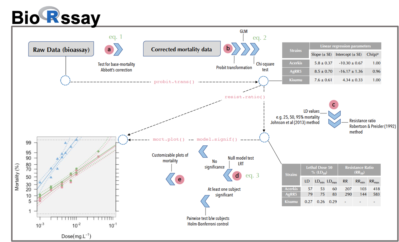
BioRssay is a comprehensive compilation of scripts in R language [11] designed to analyze dose-response relationships (or exposure-response: mortality, knock-down effect, etc.) from bioassays of one or more subjects (populations, strains, lines, tissues, cells, etc.). This package provides a complete analytic workflow from data quality assessment to statistical analyses and data visualization (see Fig. 1).
a. In the first step, the base mortality in the controls (i.e. without the stimulus to be tested) is taken into account to control for the mortality (or effect) associated with the experiment itself, regardless of the exposure. Data are adjusted following Abbott's formula using a maximum likelihood approach (optim function, method “L-BFGS-B”, stats R package[11]), to estimate correction factors (Eq. 1), while taking into account heterogeneity in the mortality rates between replicates (see example in Table 1) [12]:
\(1- \frac{{m}_{T}}{{m}_{C}}\) Eq. 1,
where mT and mC are the survival rates in the treatments and the controls, respectively. By default, the correction is applied if mortality in the control is higher than 5%, but any threshold can be specified.
b. Data are then probit-transformed and analyzed using a generalized linear model (probit-link function). The coefficients of the linear regressions (i.e. slope and intercept, with their standard errors) are reported (see example in Table 2). These coefficients are used to test the linearity of the log-dose response for each subject using a chi-square test of homogeneity between model predictions and probit-transformed data (Eq. 2); significant deviations from linearity may for example reflect mixed populations, or a threshold effect.
\({\chi }^{2}=\sum \frac{{(observed-predicted)}^{2}}{predicted}\) Eq. 2,
c. By default, lethal doses, LD (aka lethal concentrations, LC), are computed at 25%, 50%, and 95% of mortality with their corresponding 95% confidence intervals (CI), following the approach developed by Johnson et al. [10] from Finney [11], which allows taking data heterogeneity into account (Table 1); otherwise, any level of LD and CI can be specified by the user (Table 2). Resistance ratio (RR) with 95% confidence intervals are calculated according to Robertson and Preisler [13]. They measure the magnitude of the difference in dose-response of two subjects when exposed to the same stimulus. For a given LD (LD25, 50, and 95 by default), the LD of a focal subject is divided by the LD of the subject with the lowest one (usually a susceptible reference, Table 2).
d. When different subjects (population, strains, lines, etc.) are exposed to the same stimulus, we offer the possibility to test whether they present significant differences in their responses. A likelihood ratio test (LRT) is conducted to compare a null model assuming that all the data come from the same subject, where the dose is the only explanatory variable (Eq. 3), with a model considering the dose nested in the subject effect (Eq. 4).
\({y}_{i} = {a}_{i} + {\epsilon }_{i}\) Eq. 3, and \({y}_{ij} = {{\alpha }_{i}+\beta }_{j}+{\gamma }_{ij}+ {\epsilon }_{ij}\) Eq. 4,
where \(y\) is the mortality rate measured in sample i from subject j, exposed to a dose \(\alpha\), and where \(\beta\) is the subject-specific fixed-effect, \(\gamma\) is the interaction between \(\alpha\) (dose) and \(\beta\) (subject) effects and \(\epsilon\) is the error term following a quasi-binomial distribution. If the two models are significantly different (i.e. at least two subjects show differing responses either in magnitude of the response and / or slope) and that there are more than two subjects, pairwise comparisons (LRT) are implemented to test for statistical significance of the difference between all pairs of subjects; the Holm-Bonferroni method is used to control for the family-wise error inherent to multiple testing [14].
Note that if at least one of the subjects failed the linearity test described above (point b.), the validity of comparing the slope of the dose-mortality response is, at best, highly questionable (not recommended). If many subjects are present and only one (few) fails the linearity tests, we do recommend removing this (these) specific subject(s) before conducting the test.
e. Customizable (e.g. colors, symbols, title) plots of the probit-transformed regressions are drawn (Fig. 2A and B). By default, if the probit-transformed response significantly deviates from linear regression, the data are connected by segments and the regression and associated CI are not plotted (e.g. Figure 2B, Acerkis, red, and AgRR5, green, strains). Confidence intervals around the regressions can be removed or added, and users can specify any levels of CI.
Package accessibility and concluding remark
The package is available freely on GitHub at https://github.com/milesilab/BioRssay (https://doi.org/10.5281/zenodo.5172072). We also provide a comprehensive workflow and tutorials, from data preparation to the interpretation of the results, in a dedicated GitHub page https://milesilab.github.io/BioRssay/. Further, the package carries example data sets for self-tests and more data can be downloaded at https://github.com/milesilab/DATA. The code is maintained by Piyal Karunarathne ([email protected]). For suggestions or further development please contact the corresponding authors, P. Labbé and P. Milesi.
The BioRssay package can be installed in the R environment using the following code:
if (!requireNamespace("devtools", quietly = TRUE))
install.packages("devtools")
devtools::install_github("milesilab/BioRssay")