Plant materials, seedling establishment, and experimental design: Seeds from a single, inbred oilseed sunflower line (HA412-HO; PI 642777) were obtained from the North Central Regional Plant Introduction Station (NCRPIS) in Ames, IA. Seeds were planted 1.5 cm deep in individual 50 mL Falcon tubes that had been pre-drilled with two ⅛-inch holes 2 cm from the base to allow drainage. The growth substrate was a mixture of sand and Turface (3:1, v/v; Oldcastle APG Northeast, Inc., Manassas, VA). The tubes were then placed in a plant growth room where the seedlings were maintained for 20 days following germination under one of 5 differential treatments (i.e., control plus 4 stress treatments; see below). Throughout the experiment, the temperature was kept at 20˚C with a 16h:8h day:night cycle. All individuals were arranged in a randomized block design with two blocks and 11 biological replicates per treatment (5-6 per block; n = 55 seedlings total). Six replicates per treatment (three per block) were randomly designated for destructive phenotypic analyses. The remaining five replicates per treatment (2-3 per block) were designated for transcriptomic profiling, with all leaf and root tissues being harvested separately, frozen in liquid nitrogen, and stored at -80˚C prior to RNA extraction.
Treatment implementation
Upon planting, the control plants plus all individuals from the three water-related stresses were top-watered daily with a solution of deionized (DI) water and supplemental nutrients in the form of one g/L of Jack’s All Purpose 20-20-20 aqueous mix (J.R. Peters, Inc., Allentown, PA) for 10 days to facilitate seedling establishment. Following establishment, the control seedlings were maintained as above. The water-related stresses were implemented at the V2 stage of sunflower development (Schneiter and Miller, 1981) as a repeated dry-down to mimic drought stress through top-down soil drying, an osmotic challenge to limit water uptake using polyethylene glycol (PEG-6000, 8.25% by volume, which is sufficient to induce an osmotic challenge of -0.25 MPa; Masalia et al., 2018), and salt (NaCl, 100 mM) stress. In the repeated dry-down, the seedlings were transitioned from daily watering to watering with the control solution on alternate days. This decrease in frequency was sufficient to induce visible symptoms of water limitation (i.e., the seedlings began to wilt prior to re-watering) without causing mortality.
In the PEG and salt scenarios, the seedlings were transitioned to watering with treatment solutions containing the appropriate amount of PEG or salt with one g/L of Jack’s All Purpose 20-20-20 aqueous solution dissolved in DI water. All individuals were top-watered with their respective treatment solutions to bring their growth substrate to full capacity in 50mL cone-shaped containers. Osmotic stress, particularly when mediated via high molecular weight polymers such as PEG, has been a generally accepted approach for inducing water limitation in a uniform and repeatable way (e.g., Badr et al., 2020; Boureima et al., 2011; Cui et al., 2015; Fulda et al., 2011; Hadiarto and Tran, 2011; Li et al., 2021; Lian et al., 2004; Reza Yousefi et al., 2020) while minimizing toxicity effects (Oertli, 1985; Verslues et al., 2006, but see Jackson, 1962). In contrast, NaCl not only influences water uptake, but also has the potential to enter cellular pores and elicit toxic effects (Jackson, 1962; Leshem, 1966; Plaut and Federman, 1985). These differential treatments were maintained for 10 days following establishment, for a total of 20 days of seedling growth.
The individuals subjected to low-nutrient stress were top-watered daily with DI water to bring their growth substrate to full capacity, but were not provided with supplemental nutrients at any time during the experiment. This resulted in a generalized nutrient deficit relative to control conditions, similar to what might be encountered in highly degraded soils limited in nitrogen, phosphorus, calcium, or other micronutrients. Previous work has shown that this low-nutrient treatment limits growth in sunflower, but does not prevent them from completing their lifecycle (Bowsher et al., 2017).
Phenotypic measurements
A total of 21 morphological and physiological traits were measured for each phenotyped individual at the V2 stage of sunflower development after each treatment. As detailed below, these included leaf, stem, and root traits, as well as overall biomass production.
Overall plant performance
Total biomass, which served as an integrated metric of overall plant performance, was calculated as the sum of the dried leaf, stem, and root tissue (see below). Organ biomass fractions were also determined from these data as proportions of total biomass.
Leaf traits
Ten days after the start of the experiment, corresponding to initiation of the water-related stress treatments, the most recently developed leaf pair was tagged with string. Upon harvest, the next higher leaf pair was designated for measurements. This approach ensured that the leaves of interest were produced following the implementation of the stresses. One leaf from this pair was used to estimate chlorophyll concentration and relative water content; the other leaf was removed and scanned with a CanoScan 8800F scanner (Canon USA, Inc., Melville, NY) at 600 dpi, and dried for biomass estimation and isotope analyses.
An in situ optical measure of chlorophyll concentration per unit leaf area was assessed using an Apogee MC-100 chlorophyll content meter (Apogee Instruments, Logan, UT). Two readings were taken for each leaf from different parts of the leaf lamina and averaged. A leaf disc was taken using a ¼-inch diameter hole punch and used to assess leaf relative water content (RWC), which serves as an indicator of plant water status (Lawlor and Cornic, 2002). This was calculated as (FM-DM)/(HM-DM), where FM was fresh mass at the time of collection, HM was hydrated mass (estimated after hydrating the leaf punches for 24 hours), and DM was dry mass, estimated after drying the leaf punches at 60˚C for 72 hours in a forced-air drying oven (Smart, 1974).
Leaf area estimates were obtained from the scanned images using ImageJ (Schneider et al., 2012). After scanning, the leaves were dried as above and weighed to estimate dry biomass, which was used to calculate leaf mass per area (LMA). The dried leaves were then ground into a fine, homogenous powder using a Thomas Model 4 Wiley ball mill (Thomas Scientific, Swedesboro, NJ) for stable isotope analyses, which were performed at the University of Georgia’s Stable Isotope Ecology Laboratory (http://siel.uga.edu/). This yielded estimates of total percent leaf carbon and leaf nitrogen, as well as carbon and nitrogen isotope composition (δ13C, δ15N).
All remaining leaves were dried as above and weighed, and all leaf weights for a given seedling were summed to provide an overall estimate of leaf biomass. Leaf mass fraction (LMF) was then calculated as leaf biomass divided by total biomass.
Stem traits
After harvest, stem height and diameter were measured using Fowler 6"/150mm Ultra-Cal IV Electronic Calipers (Fowler Tools and Instruments, Newton, MA). Stem diameter was measured just above soil level. Stem tissue was then dried as above and weighed to estimate stem biomass. Stem mass fraction (SMF) was then calculated as stem biomass divided by total biomass.
Root traits: Seedlings were gently uprooted, and root tissue was rinsed to remove soil substrate. Intact roots were patted dry, fanned out, and placed in a vertical orientation on a matte black cloth for imaging. A coin (US penny; 19.05 mm diameter) was placed next to each root system for scale. Photos were then taken with a 12 megapixel camera from a fixed distance of 175 mm and uploaded to the Digital Imaging of Root Traits (DIRT) pipeline (Das et al., 2015) with a masking threshold calibration of 5.00. The following traits were assessed: number of tip paths and rooting depth skeleton (both are “common traits” in DIRT); roots seg 1 and 2, number of adventitious and basal roots, hypocotyl diameter, and taproot diameter (all of these are “dicot traits” in DIRT). Following imaging, the roots were dried as above and weighed to estimate root biomass. Root mass fraction (RMF) was then calculated as root biomass divided by total biomass.
Statistical analysis of phenotypic traits
All analyses of phenotypic data were performed in R v4.04 (R Core Team, 2013). To protect against violations of the assumption of normality, a nonparametric Kruskal-Wallis test used to test for an overall treatment effect while controlling for block effects. A pairwise Wilcoxon test with an FDR P-adjustment method (Benjamini and Hochberg, 1995) was used to test for differences in phenotypic responses between stress treatments for all traits with a significant (P < 0.05) treatment effect. Finally, two principal component analyses (PCAs) were performed; one of these analyses used the full set of traits (n = 21) to assess the clustering of treatments across trait space, and the other used just the size-independent traits (n = 10) to capture treatment clustering without the influence of metrics related to overall growth and performance. The bioconductor package pcaMethods (Stacklies et al., 2007) was used to impute values for 11 missing data points out of 630 individual measurements.
RNA extraction and sequencing: Tissue samples from five biological replicates for each of the five treatments were used for total RNA isolation, with replicates maintained as separate samples (i.e., they were not pooled). Leaf and root tissue were ground separately in liquid nitrogen using a pre-chilled mortar and pestle to produce a fine powder (ca. 100 µg per sample). Total RNA was then extracted from the ground samples using the RNeasy Mini Kit (Qiagen, Inc., Germantown, MD). RNA extractions were treated to remove DNA contamination using a TURBO DNA-free kit (ThermoFisher Scientific, Waltham, MA). The quality and quantity of each RNA sample was assessed using a NanoDrop 2000 (ThermoFisher Scientific) and an Agilent 2100 Bioanalyzer (Agilent Technologies, Alpharetta, GA). Only RNA samples with 260/280 ratios from 1.8 to 2.1, 260/230 ratios ≥ 2.0, and RNA integrity number (RIN) values greater than 7.5 were used for subsequent analyses. Approximately 1 µg of total RNA from each sample was used to construct sequencing libraries using the KAPA Stranded mRNA-Seq Kit (KAPA Biosystems, Wilmington, MA). Thirty-eight individual libraries passing our quality control standards were generated (control: four leaf, three root; dry-down: four leaf, three root; PEG: four leaf, three root; salt: five leaf, five root; low-nutrient: four leaf, three root) and sequenced (paired-end, 75 bp reads) at the Georgia Genomics and Bioinformatics Core (http://dna.uga.edu/) on an Illumina NextSeq (Illumina, San Diego, CA).
Sequence assembly, read mapping, and gene expression analyses: RNAseq data was processed using a custom bioinformatics pipeline (https://github.com/EDitt/Sunflower_RNAseq) as implemented in Barnhart et al., 2021. Raw sequence reads were processed by removing reads containing adapter sequences, as well as unknown or low-quality bases, using Trimmomatic v0.36 (Bolger et al., 2014) with its default settings. Cleaned reads were aligned to the cultivated sunflower reference genome (XRQv2.0; Badouin et al., 2017) using STAR v2.7.9a (Dobin et al., 2013) with default parameters. Next, gene expression abundances were calculated per library using RSEM v1.3.3 (Li and Dewey, 2011) with default parameters. Finally, the Bioconductor program edgeR v3.34.0 (Robinson et al., 2010) was used to produce normalized read counts via TMM normalization and to identify differentially expressed genes (DEGs) across treatments and tissue types. The model used to identify DEGs separated samples by tissue and stress type then compared the expression against control samples of the same tissue type. For a gene to be considered for differential expression analysis, it had to meet a minimum expression threshold of 1 count-per-million in 2 or more libraries within a tissue/treatment group. A total of 39,042 genes were retained for this analysis. A false discovery rate (FDR) of ≤ 0.05 was used as the threshold for identifying DEGs. At this point, five outlier libraries (P5L, P3R, S1L, C2L, DD3L) were identified based on multidimensional scaling plots and removed from subsequent analyses (Supplementary figure S1A and S1B). These corresponded to the five samples with the fewest number of reads in the data set. All DEGs were then classified based on tissue specificity (i.e., leaf-specific, root-specific, or shared) as well as stress specificity (i.e., stress-specific or shared by a particular combination of stresses).
To test whether the number of unique genes found in each stress combination was more or less than expected by chance, we took random samples of genes that passed the minimum expression threshold for each stress 1000 times and then calculated the overlap. The number of random genes sampled for each stress was equal to the number of true DEGs found for that stress. The number of unique genes in each stress combination from each random sample was then used to create a distribution from the 1000 samples for the true results to be tested against. P-values were estimated by finding the percentile for which the true value fell in each distribution and multiplying it by 2 for an upper and lower two-tailed test. To further explore the similarity of the transcriptional responses of each tissue type to the various stress scenarios, MDS plots were created from TMM normalized counts for different gene and sample sets using edgeR.
Gene co-expression network construction
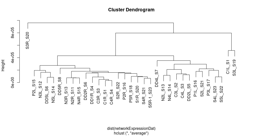
We built a signed gene co-expression network using WGCNA v1.70-3 (Langfelder and Horvath, 2008). All genes used for the differential expression were retained for the network construction, with the exception of 11 genes that did not meet the default variance requirements of WGCNA. Three additional outlier samples were removed based upon distance matrix clustering recommended by WGCNA (Supplementary figure S3). A soft-thresholding power of 14 was used to build a signed network given our number of samples and the lack of scale-free topology association due to variance in the data caused by the treatment design as recommended by the WGCNA manual. We then used the automatic 1-step blockwise network construction approach with a maximum block size of 20,000, splitting the data into two blocks, to generate the topological overlap matrix. We did not determine correlations between the co-expression network and the phenotypes measured as RNA was not extracted from the same plants for which we (destructively) measured phenotypes. Correlations were determined between network modules, treatments, and tissues. To test for the enrichment of genes belonging to specific modules within DEG intersections, we first simulated 1,000 co-expression networks by randomly assigning genes to modules of the same sizes as those in the network built from our experimental data. We then asked which simulated module each DEG belonged to and created a distribution of module membership statistics. Lastly, for each set of DEGs, we asked if there were more or less genes belonging to each module than expected by chance and estimated P-values from the distribution of the simulated data.
Classification and GO term enrichment of DEGs: A list of gene annotations and a gene ontology (GO) index were downloaded for the XRQv2.0 reference genome (http://www.heliagene.org/). A GO enrichment analysis was then performed for all DEGs in each tissue, stress combination, and network module using GOseq v.1.44.0 (Young et al., 2010) to normalize for gene length bias. A significance threshold of P < 0.05 was used to determine the significance of GO term enrichment after a multiple hypothesis correction using the Benjamini-Hochberg methodology (Benjamini and Hochberg, 1995).